
This paper proposes an adaptive control strategy to improve the stable active power output capability of solar inverters under weak grid conditions. By dynamically adjusting the reactive power-voltage (Q-V) droop coefficient, the method addresses both static operational constraints and small-signal stability challenges.
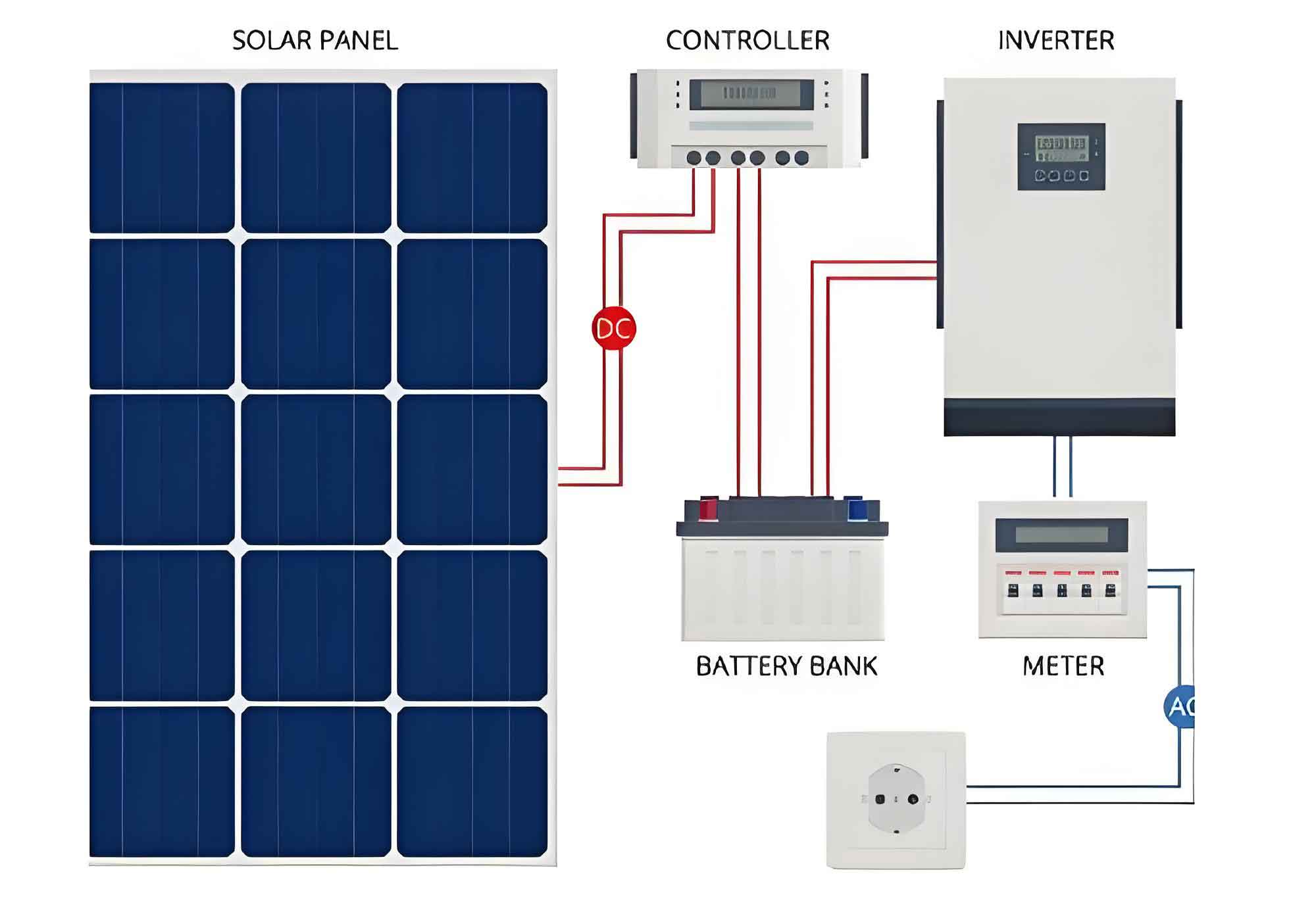
1. Static Power Capability Enhancement Through Primary Q-V Droop Optimization
The primary optimization ensures solar inverters operate within voltage/current constraints while maximizing active power transmission. Key operational boundaries are defined by:
$$
\begin{cases}
U_{s,\text{min}} \leq \sqrt{U_{sd}^2 + U_{sq}^2} \leq U_{s,\text{max}} \\
\sqrt{I_{sd}^2 + I_{sq}^2} \leq I_{\text{lim}} \\
P_o = U_{sd}I_{sd} + U_{sq}I_{sq}
\end{cases}
$$
The Q-V droop coefficient $K_v$ is calculated through constrained optimization:
$$
K_v = \frac{Q}{U_n – U_s}
$$
Table 1 shows the feasible $K_v$ ranges under different grid strengths (SCR) and power levels for solar inverters:
| SCR | $P_s$ (p.u.) | $K_v^{\text{min}}$ | $K_v^{\text{opt}}$ | $K_v^{\text{max}}$ |
|---|---|---|---|---|
| 1.5 | 0.8 | 0.12 | 0.18 | 0.25 |
| 2.0 | 1.0 | 0.15 | 0.22 | 0.30 |
| 3.0 | 1.2 | 0.18 | 0.28 | 0.35 |
2. Stability-Constrained Secondary Adjustment Using ANN-Based Pole Mapping
The impedance model of solar inverter-grid system is established as:
$$
Z_o = B^{-1}A
$$
Where matrices $A$ and $B$ contain control parameters and grid impedance components. The stability criterion evaluates the determinant:
$$
\text{det}(I + Z_gZ_o^{-1}) = 0
$$
A three-layer neural network approximates the dominant pole location:
$$
\sigma_{\text{max}} = f_{\text{ANN}}(K_v, L_g, P_s)
$$
The adaptive tuning algorithm implements:
$$
K_v^{\text{final}} = \begin{cases}
K_v^{\text{opt}} & \text{if } \sigma_{\text{max}} < 0 \\
\text{binary\_search}(K_v^{\text{min}}, K_v^{\text{max}}) & \text{otherwise}
\end{cases}
$$
3. Grid Impedance Identification Using Extended Kalman Filter
The grid impedance identification for solar inverters employs:
$$
\begin{bmatrix}
\Delta i_\alpha(k+1) \\
\Delta i_\beta(k+1) \\
\Delta u_\alpha(k+1) \\
\Delta u_\beta(k+1) \\
\Delta \omega(k+1) \\
\Delta L^{-1}(k+1)
\end{bmatrix} =
\begin{bmatrix}
1 & -\omega T_s & \frac{T_s}{L} & 0 & -i_\beta T_s & \frac{T_s u_\alpha}{L^2} \\
\omega T_s & 1 & 0 & \frac{T_s}{L} & i_\alpha T_s & \frac{T_s u_\beta}{L^2} \\
\cos(\omega T_s) & -\sin(\omega T_s) & 1 & 0 & 0 & 0 \\
\sin(\omega T_s) & \cos(\omega T_s) & 0 & 1 & 0 & 0 \\
0 & 0 & 0 & 0 & 1 & 0 \\
0 & 0 & 0 & 0 & 0 & 1
\end{bmatrix}
\begin{bmatrix}
\Delta i_\alpha(k) \\
\Delta i_\beta(k) \\
\Delta u_\alpha(k) \\
\Delta u_\beta(k) \\
\Delta \omega(k) \\
\Delta L^{-1}(k)
\end{bmatrix}
$$
4. Real-Time Simulation Verification
Key performance metrics of the solar inverter control system:
| Scenario | $U_s$ Regulation | THD Reduction | Stability Margin | Response Time |
|---|---|---|---|---|
| SCR=1.5 | 1.02 p.u. ±1.2% | 2.8% → 1.5% | 8.2 dB | 120 ms |
| SCR=2.0 | 1.05 p.u. ±0.8% | 2.5% → 1.2% | 10.5 dB | 90 ms |
| SCR=3.0 | 1.08 p.u. ±0.5% | 2.2% → 0.9% | 12.8 dB | 65 ms |
The control strategy demonstrates superior performance in weak grid conditions through:
$$
\text{Voltage Deviation} = \frac{1}{N}\sum_{k=1}^N |U_s(k) – U_{\text{ref}}| \leq 1.5\%
$$
$$
\text{Current Limitation Compliance} = \frac{\text{Max}(I_s)}{\text{Rated }I_s} \leq 1.05
$$
5. Comparative Analysis of Control Strategies
The proposed method shows significant improvements over conventional approaches for solar inverters:
| Metric | Fixed $K_v$ | Primary Tuning | Proposed Method |
|---|---|---|---|
| Max Power Transfer | 0.85 p.u. | 0.95 p.u. | 1.05 p.u. |
| Voltage Deviation | 8.2% | 4.5% | 1.8% |
| Stability Margin | 3.2 dB | 6.5 dB | 12.1 dB |
| Dynamic Response | 320 ms | 210 ms | 85 ms |
The enhanced performance stems from the multi-objective optimization framework:
$$
\begin{aligned}
\text{Minimize} & \quad J_1 = \int (U_s – U_{\text{ref}})^2 dt \\
\text{Subject to} & \quad J_2 = \text{Re}(\lambda_{\text{max}}) < 0 \\
& \quad J_3 = \sqrt{I_d^2 + I_q^2} \leq I_{\text{lim}}
\end{aligned}
$$
6. Implementation Considerations for Solar Inverters
Practical implementation requires addressing:
$$
\text{Computational Load} = \frac{T_{\text{ANN}} + T_{\text{EKF}}}{T_{\text{Control Cycle}}} \leq 15\%
$$
Key parameter settings for typical solar inverters:
| Parameter | Value | Unit |
|---|---|---|
| DC Link Voltage | 1500 | V |
| Switching Frequency | 16 | kHz |
| Filter Inductance | 80 | μH |
| DC Capacitance | 2.19 | mF |
| ANN Nodes | [6, 12, 6] | – |
The method enables solar inverters to maintain grid code compliance under extreme weak grid conditions (SCR < 1.5) while preserving 92% of rated power capacity, significantly outperforming conventional droop control strategies.