
The accurate estimation of the State of Charge (SOC) remains a cornerstone for the safe, efficient, and reliable operation of lithium-ion batteries, especially in demanding applications such as electric vehicles and grid-scale energy storage systems. As the core of the Battery Management System (BMS), precise SOC information is critical for preventing operational hazards like overcharge and over-discharge, optimizing energy usage, and predicting battery lifespan. However, SOC is an internal state that cannot be measured directly and is influenced by complex, nonlinear electrochemical dynamics, temperature, aging, and measurement noise. Traditional methods like Coulomb counting suffer from error accumulation due to current sensor drift and uncertain initial conditions, while open-circuit voltage (OCV) methods require long rest periods impractical for real-time operation. Consequently, model-based estimation algorithms, particularly those derived from the Kalman filter (KF) framework, have become the predominant solution for achieving robust and accurate SOC estimates in real-time.
Extended Kalman Filters (EKF) linearize the nonlinear system, which can introduce significant errors for highly nonlinear systems like lithium-ion batteries. The Unscented Kalman Filter (UKF) improves upon this by using a deterministic sampling technique. However, as system dimensionality increases, the numerical stability of the UKF can degrade, potentially leading to non-positive definite error covariance matrices and filter divergence. The Cubature Kalman Filter (CKF), grounded in the third-degree spherical-radial cubature rule, offers a more rigorous framework for multidimensional integration in Bayesian filtering, often providing better accuracy and stability than the UKF. Yet, in practical implementations, especially with poor numerical conditioning or specific noise characteristics, the standard CKF can also experience numerical issues where the error covariance matrix loses its positive definiteness, leading to unreliable and divergent state estimates.
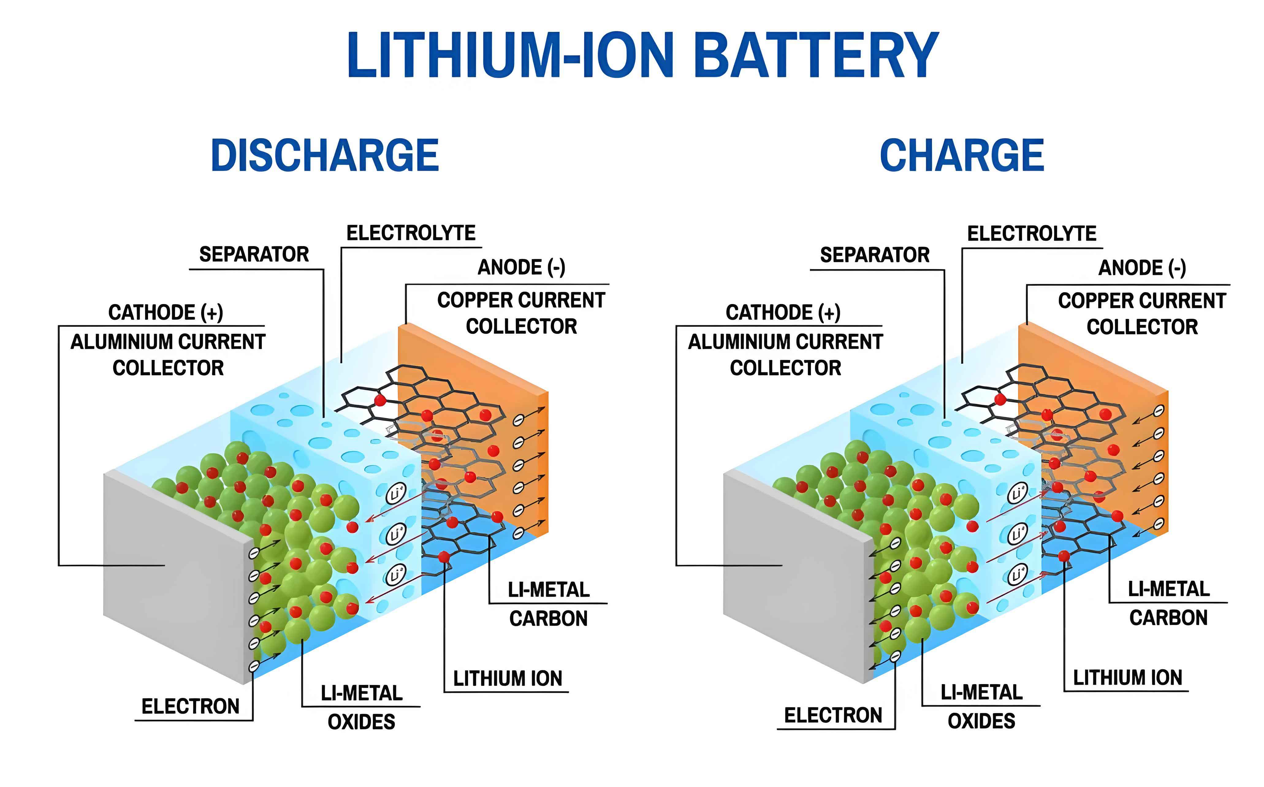
This work focuses on enhancing the numerical robustness and estimation accuracy of SOC algorithms for lithium-ion batteries. We employ a second-order RC equivalent circuit model (dual-polarization model) to capture the dynamic behavior of a lithium iron phosphate (LFP) lithium-ion battery. The model parameters are identified online using a Recursive Least Squares (RLS) algorithm. To address the potential divergence issue in the standard CKF, we implement and validate a Square-Root Cubature Kalman Filter (SRCKF). The SRCKF algorithm propagates the square-root factors of the error covariance matrices instead of the full matrices themselves, inherently ensuring positive semi-definiteness through the use of efficient QR decompositions and Cholesky updates. This approach significantly improves numerical stability. Experimental results under constant current and dynamic stress test (DST) profiles demonstrate that the proposed SRCKF-based method delivers superior estimation accuracy compared to the conventional CKF, achieving a lower root mean square error (RMSE) in terminal voltage prediction and, consequently, more reliable SOC estimation for the lithium-ion battery.
Modeling of the Lithium-Ion Battery
An accurate yet computationally tractable model is essential for model-based SOC estimation. Electrochemical models, while physically detailed, are too complex for real-time BMS applications. Equivalent circuit models (ECMs) offer a favorable balance between fidelity and simplicity. For a lithium-ion battery, the second-order RC model, or dual-polarization model, effectively captures the major dynamic voltage responses: the immediate ohmic drop and the short/long-term polarization effects.
The Dual-Polarization Equivalent Circuit Model
The chosen model for the lithium-ion battery is depicted in the figure below. It consists of a voltage source representing the open-circuit voltage \(U_{oc}(SOC)\), which is a nonlinear function of the SOC, a series ohmic resistance \(R_0\), and two parallel RC networks. The first RC branch (\(R_1, C_1\)) models the short-term electrochemical polarization, while the second branch (\(R_2, C_2\)) models the long-term concentration polarization. The terminal voltage is denoted as \(U_b\), and the applied current is \(I_b\) (discharge positive, charge negative).
Applying Kirchhoff’s laws to this lithium-ion battery model yields the following dynamic equations:
$$
\frac{dU_1}{dt} = -\frac{1}{R_1 C_1}U_1 + \frac{1}{C_1} I_b
$$
$$
\frac{dU_2}{dt} = -\frac{1}{R_2 C_2}U_2 + \frac{1}{C_2} I_b
$$
$$
U_b = U_{oc}(SOC) – U_1 – U_2 – R_0 I_b
$$
where \(U_1\) and \(U_2\) are the voltages across the polarization capacitors. The state-space representation is crucial for filter design. By defining the state vector \(\mathbf{x} = [SOC, U_1, U_2]^T\), the input \(u = I_b\), and the output \(y = U_b\), and noting that \(d(SOC)/dt = -\eta I_b / Q_n\) (where \(\eta\) is coulombic efficiency and \(Q_n\) is nominal capacity), we can derive the continuous-time state-space model for the lithium-ion battery:
$$
\dot{\mathbf{x}} = \begin{bmatrix} 0 & 0 & 0 \\ 0 & -\frac{1}{R_1 C_1} & 0 \\ 0 & 0 & -\frac{1}{R_2 C_2} \end{bmatrix} \mathbf{x} + \begin{bmatrix} -\frac{\eta}{Q_n} \\ \frac{1}{C_1} \\ \frac{1}{C_2} \end{bmatrix} u
$$
$$
y = U_{oc}(\mathbf{x}_1) – \begin{bmatrix} 0 & 1 & 1 \end{bmatrix} \mathbf{x} – R_0 u
$$
For digital implementation in a BMS, the model must be discretized. Using a zero-order hold on the input with sampling time \(T_s\), the discrete-time state-space model becomes:
$$
\mathbf{x}_{k+1} = \begin{bmatrix} 1 & 0 & 0 \\ 0 & e^{-T_s/(R_1 C_1)} & 0 \\ 0 & 0 & e^{-T_s/(R_2 C_2)} \end{bmatrix} \mathbf{x}_k + \begin{bmatrix} -\frac{\eta T_s}{Q_n} \\ R_1(1-e^{-T_s/(R_1 C_1)}) \\ R_2(1-e^{-T_s/(R_2 C_2)}) \end{bmatrix} u_k + \mathbf{w}_k
$$
$$
y_k = U_{oc}(SOC_k) – U_{1,k} – U_{2,k} – R_0 u_k + v_k
$$
where \(\mathbf{w}_k\) and \(v_k\) represent the process and measurement noise, respectively, assumed to be zero-mean white Gaussian sequences with covariances \(\mathbf{Q}\) and \(R\).
Open-Circuit Voltage (OCV) Characterization
The relationship \(U_{oc}(SOC)\) is a critical, highly nonlinear component of the lithium-ion battery model. Its accuracy directly impacts the SOC estimation performance. Due to hysteresis, the OCV depends on the immediate history (charge or discharge). A common practice is to use the average of charge and discharge OCV curves. The OCV-SOC relationship is determined experimentally by performing a low-current charge/discharge test with long relaxation periods at regular SOC intervals to allow the terminal voltage to settle to its equilibrium OCV.
For the LFP lithium-ion battery used in this study, the averaged OCV data points were fitted using an 8th-order polynomial, which provided the best compromise between fit accuracy and model complexity. The resulting function is:
$$
U_{oc}(SOC) = -272.6 SOC^8 + 1236.4 SOC^7 – 2238.6 SOC^6 + 2225.3 SOC^5 – 1274.5 SOC^4 + 429.2 SOC^3 – 79.5 SOC^2 + 8.9 SOC + 3.1427
$$
This polynomial provides a continuous and differentiable representation of the OCV-SOC nonlinearity essential for the filter algorithms.
Online Parameter Identification via RLS
The model parameters \(\theta = [R_0, R_1, C_1, R_2, C_2]\) are not constant for a lithium-ion battery; they vary with SOC, temperature, and state of health (SOH). Therefore, online identification is necessary for adaptive and accurate estimation. We employ the Recursive Least Squares (RLS) algorithm with forgetting factor for this purpose.
First, the continuous-time transfer function from \(I_b(s)\) to \(E_L(s)=U_{oc}(s)-U_b(s)\) is derived from the model equations:
$$
\frac{E_L(s)}{I_b(s)} = -\left( R_0 + \frac{R_1}{1+R_1 C_1 s} + \frac{R_2}{1+R_2 C_2 s} \right)
$$
Applying the bilinear transformation \(s = \frac{2}{T_s} \frac{1-z^{-1}}{1+z^{-1}}\) converts this to a discrete-time transfer function:
$$
G(z^{-1}) = \frac{b_3 + b_4 z^{-1} + b_5 z^{-2}}{1 – b_1 z^{-1} – b_2 z^{-2}}
$$
This corresponds to the Auto-Regressive with eXogenous input (ARX) model difference equation:
$$
E_{L,k} = b_1 E_{L,k-1} + b_2 E_{L,k-2} + b_3 I_{b,k} + b_4 I_{b,k-1} + b_5 I_{b,k-2}
$$
The RLS algorithm then identifies the parameter vector \(\hat{\mathbf{\phi}}_k = [b_1, b_2, b_3, b_4, b_5]^T\). The steps are summarized below:
RLS Algorithm Steps:
1. Initialize: \(\hat{\mathbf{\phi}}_0 = \mathbf{0}\), \(\mathbf{P}_0 = \lambda^{-1} \mathbf{I}\), where \(\lambda\) is a large constant (e.g., 1000) and \(\mathbf{I}\) is the identity matrix. Set forgetting factor \(0 < \gamma \leq 1\).
2. Construct Data Vector: For each time step \(k\), form the regression vector:
$$
\mathbf{\psi}_k = [E_{L,k-1}, E_{L,k-2}, I_{b,k}, I_{b,k-1}, I_{b,k-2}]^T
$$
3. Calculate Gain:
$$
\mathbf{K}_k = \frac{\mathbf{P}_{k-1} \mathbf{\psi}_k}{\gamma + \mathbf{\psi}_k^T \mathbf{P}_{k-1} \mathbf{\psi}_k}
$$
4. Update Estimate:
$$
\hat{\mathbf{\phi}}_k = \hat{\mathbf{\phi}}_{k-1} + \mathbf{K}_k (E_{L,k} – \mathbf{\psi}_k^T \hat{\mathbf{\phi}}_{k-1})
$$
5. Update Covariance:
$$
\mathbf{P}_k = \gamma^{-1} (\mathbf{P}_{k-1} – \mathbf{K}_k \mathbf{\psi}_k^T \mathbf{P}_{k-1})
$$
6. Recover Physical Parameters: From the estimated \(\hat{\mathbf{\phi}}_k\), the original lithium-ion battery model parameters \(\{R_0, R_1, C_1, R_2, C_2\}\) can be recovered algebraically using the following relationships derived from the bilinear transformation coefficients:
Let intermediate variables be calculated as:
$$
\Delta = 1 – b_1 – b_2
$$
$$
A = \frac{T_s (1 + b_2)}{2 \Delta}
$$
$$
B = \frac{T_s^2 (1 + b_1 – b_2)}{8 \Delta}
$$
Then the time constants and resistances are:
$$
\tau_1 \tau_2 = B, \quad \tau_1 + \tau_2 = \frac{A}{2}
$$
$$
R_0 = \frac{b_4 – b_3 – b_5}{4 \Delta}
$$
$$
R_0 + R_1 + R_2 = -\frac{b_3 + b_4 + b_5}{2 \Delta}
$$
$$
R_0 (\tau_1 + \tau_2) + R_1 \tau_2 + R_2 \tau_1 = \frac{T_s (b_5 – b_3)}{4 \Delta}
$$
Solving this system of equations yields the identified parameters for the lithium-ion battery model at each time step \(k\).
| Parameter | Symbol | Typical Estimated Range | Unit |
|---|---|---|---|
| Ohmic Resistance | \(R_0\) | \(0.01 – 0.03\) | Ω |
| Polarization Resistance 1 | \(R_1\) | \(0.005 – 0.015\) | Ω |
| Polarization Capacitance 1 | \(C_1\) | \(2000 – 6000\) | F |
| Polarization Resistance 2 | \(R_2\) | \(0.005 – 0.02\) | Ω |
| Polarization Capacitance 2 | \(C_2\) | \(5000 – 20000\) | F |
State-of-Charge Estimation Algorithms
With an identified model, the SOC estimation problem is formulated as a nonlinear state estimation task. The Cubature Kalman Filter (CKF) provides a powerful framework for this, and its square-root variant (SRCKF) enhances numerical stability for the lithium-ion battery application.
Cubature Kalman Filter (CKF) Framework
The CKF is designed to handle the nonlinear state-space model of the lithium-ion battery:
$$
\mathbf{x}_k = \mathbf{f}(\mathbf{x}_{k-1}, u_{k-1}) + \mathbf{w}_{k-1}
$$
$$
y_k = \mathbf{h}(\mathbf{x}_k, u_k) + v_k
$$
where \(\mathbf{f}(\cdot)\) and \(\mathbf{h}(\cdot)\) are the nonlinear state transition and measurement functions derived from the discretized battery model. The core idea of CKF is to approximate the prior and posterior probability distributions using a set of \(2n\) equally weighted cubature points (where \(n\) is the state dimension), which capture the mean and covariance of the state. These points are propagated through the nonlinear functions.
Standard CKF Steps:
1. Initialize: \(\hat{\mathbf{x}}_{0|0} = E[\mathbf{x}_0]\), \(\mathbf{P}_{0|0} = E[(\mathbf{x}_0 – \hat{\mathbf{x}}_{0|0})(\mathbf{x}_0 – \hat{\mathbf{x}}_{0|0})^T]\).
2. Time Update (Prediction):
a) Factorize: \(\mathbf{P}_{k-1|k-1} = \mathbf{S}_{k-1|k-1} \mathbf{S}_{k-1|k-1}^T\).
b) Generate cubature points: \( \mathbf{X}_{i, k-1|k-1} = \hat{\mathbf{x}}_{k-1|k-1} + \mathbf{S}_{k-1|k-1} \boldsymbol{\xi}_i \), where \(\boldsymbol{\xi}_i = \sqrt{n} [\mathbf{1}]_i\), and \([\mathbf{1}]\) is the set of \(n\)-dimensional unit vectors (e.g., for \(n=3\), \(\{[1,0,0]^T, [0,1,0]^T, [0,0,1]^T, [-1,0,0]^T, [0,-1,0]^T, [0,0,-1]^T\}\)).
c) Propagate points: \( \mathbf{X}^*_{i, k|k-1} = \mathbf{f}(\mathbf{X}_{i, k-1|k-1}, u_{k-1}) \).
d) Estimate predicted state and covariance:
$$
\hat{\mathbf{x}}_{k|k-1} = \frac{1}{2n} \sum_{i=1}^{2n} \mathbf{X}^*_{i, k|k-1}
$$
$$
\mathbf{P}_{k|k-1} = \frac{1}{2n} \sum_{i=1}^{2n} \mathbf{X}^*_{i, k|k-1} (\mathbf{X}^*_{i, k|k-1})^T – \hat{\mathbf{x}}_{k|k-1} \hat{\mathbf{x}}_{k|k-1}^T + \mathbf{Q}_{k-1}
$$
3. Measurement Update (Correction):
a) Factorize: \(\mathbf{P}_{k|k-1} = \mathbf{S}_{k|k-1} \mathbf{S}_{k|k-1}^T\).
b) Generate new cubature points: \(\mathbf{X}_{i, k|k-1} = \hat{\mathbf{x}}_{k|k-1} + \mathbf{S}_{k|k-1} \boldsymbol{\xi}_i\).
c) Propagate through measurement function: \(\mathbf{Y}_{i, k|k-1} = \mathbf{h}(\mathbf{X}_{i, k|k-1}, u_k)\).
d) Estimate predicted measurement and innovation covariance:
$$
\hat{y}_{k|k-1} = \frac{1}{2n} \sum_{i=1}^{2n} \mathbf{Y}_{i, k|k-1}
$$
$$
\mathbf{P}_{yy, k|k-1} = \frac{1}{2n} \sum_{i=1}^{2n} \mathbf{Y}_{i, k|k-1} \mathbf{Y}_{i, k|k-1}^T – \hat{y}_{k|k-1} \hat{y}_{k|k-1}^T + R_k
$$
$$
\mathbf{P}_{xy, k|k-1} = \frac{1}{2n} \sum_{i=1}^{2n} \mathbf{X}_{i, k|k-1} \mathbf{Y}_{i, k|k-1}^T – \hat{\mathbf{x}}_{k|k-1} \hat{y}_{k|k-1}^T
$$
e) Compute Kalman gain, state estimate, and covariance:
$$
\mathbf{K}_k = \mathbf{P}_{xy, k|k-1} \mathbf{P}_{yy, k|k-1}^{-1}
$$
$$
\hat{\mathbf{x}}_{k|k} = \hat{\mathbf{x}}_{k|k-1} + \mathbf{K}_k (y_k – \hat{y}_{k|k-1})
$$
$$
\mathbf{P}_{k|k} = \mathbf{P}_{k|k-1} – \mathbf{K}_k \mathbf{P}_{yy, k|k-1} \mathbf{K}_k^T
$$
While theoretically sound, the standard CKF requires explicit computation and inversion of the covariance matrices \(\mathbf{P}_{k|k-1}\) and \(\mathbf{P}_{yy, k|k-1}\). In finite-precision arithmetic, especially with ill-conditioned data or poor tuning, these matrices can lose their positive definiteness due to round-off errors in the subtraction operations, leading to filter divergence for the lithium-ion battery SOC estimation.
Square-Root Cubature Kalman Filter (SRCKF) Algorithm
The SRCKF addresses the numerical instability by propagating the square-root factors of the covariance matrices directly, using orthogonal transformations (QR decomposition) and the Cholesky update. This ensures that the covariance matrices remain symmetric and positive semi-definite by construction. The key modifications to the CKF are the use of the qr() and cholupdate() operations.
SRCKF Algorithm Steps:
1. Initialize: \(\hat{\mathbf{x}}_{0|0} = E[\mathbf{x}_0]\), \(\mathbf{S}_{0|0} = \text{chol}(E[(\mathbf{x}_0 – \hat{\mathbf{x}}_{0|0})(\mathbf{x}_0 – \hat{\mathbf{x}}_{0|0})^T])\), where \(\text{chol}(\cdot)\) denotes the Cholesky decomposition. Set \(\mathbf{S}_Q = \text{chol}(\mathbf{Q})\) and \(S_R = \sqrt{R}\).
2. Time Update (Prediction):
a) Evaluate cubature points as in CKF: \(\mathbf{X}_{i, k-1|k-1} = \hat{\mathbf{x}}_{k-1|k-1} + \mathbf{S}_{k-1|k-1} \boldsymbol{\xi}_i\).
b) Propagate points: \(\mathbf{X}^*_{i, k|k-1} = \mathbf{f}(\mathbf{X}_{i, k-1|k-1}, u_{k-1})\).
c) Estimate predicted state:
$$
\hat{\mathbf{x}}_{k|k-1} = \frac{1}{2n} \sum_{i=1}^{2n} \mathbf{X}^*_{i, k|k-1}
$$
d) Compute the square-root of the predicted error covariance. First, form the weighted centered matrix:
$$
\mathbf{X}^*_{k|k-1} = \frac{1}{\sqrt{2n}} [\mathbf{X}^*_{1, k|k-1} – \hat{\mathbf{x}}_{k|k-1}, \mathbf{X}^*_{2, k|k-1} – \hat{\mathbf{x}}_{k|k-1}, …, \mathbf{X}^*_{2n, k|k-1} – \hat{\mathbf{x}}_{k|k-1}]
$$
Then, perform a QR decomposition on the compound matrix:
$$
\mathbf{T} = \text{qr}\left( [\mathbf{X}^*_{k|k-1}, \quad \mathbf{S}_Q]^T \right)
$$
The matrix \(\mathbf{T}\) is upper triangular. The square-root of the prior covariance is obtained from the first \(n\) rows and \(n\) columns of \(\mathbf{T}^T\):
$$
\mathbf{S}_{k|k-1} = \mathbf{T}^T (1:n, 1:n)
$$
3. Measurement Update (Correction):
a) Generate cubature points: \(\mathbf{X}_{i, k|k-1} = \hat{\mathbf{x}}_{k|k-1} + \mathbf{S}_{k|k-1} \boldsymbol{\xi}_i\).
b) Propagate through measurement function: \(\mathbf{Y}_{i, k|k-1} = \mathbf{h}(\mathbf{X}_{i, k|k-1}, u_k)\).
c) Estimate predicted measurement:
$$
\hat{y}_{k|k-1} = \frac{1}{2n} \sum_{i=1}^{2n} \mathbf{Y}_{i, k|k-1}
$$
d) Compute the square-root of the innovation covariance. Form the weighted matrices:
$$
\mathbf{Y}_{k|k-1} = \frac{1}{\sqrt{2n}} [\mathbf{Y}_{1, k|k-1} – \hat{y}_{k|k-1}, \mathbf{Y}_{2, k|k-1} – \hat{y}_{k|k-1}, …, \mathbf{Y}_{2n, k|k-1} – \hat{y}_{k|k-1}]
$$
$$
\mathbf{X}_{k|k-1} = \frac{1}{\sqrt{2n}} [\mathbf{X}_{1, k|k-1} – \hat{\mathbf{x}}_{k|k-1}, \mathbf{X}_{2, k|k-1} – \hat{\mathbf{x}}_{k|k-1}, …, \mathbf{X}_{2n, k|k-1} – \hat{\mathbf{x}}_{k|k-1}]
$$
Perform a QR decomposition:
$$
\begin{bmatrix} \mathcal{Y} \\ \mathcal{X} \end{bmatrix} = \text{qr}\left( \begin{bmatrix} \mathbf{Y}_{k|k-1} & S_R \\ \mathbf{X}_{k|k-1} & \mathbf{0} \end{bmatrix}^T \right)^T
$$
The matrix \(\mathcal{Y}\) is upper triangular. The square-root of the innovation covariance is:
$$
\mathbf{S}_{yy, k|k-1} = \mathcal{Y}(1:1, 1:1) \quad \text{(a scalar for single output)}
$$
The cross-weighting matrix is:
$$
\mathcal{P}_{xy, k|k-1} = \mathcal{X}(1:n, 1:1)
$$
e) Compute Kalman gain and update state square-root factor:
$$
\mathbf{K}_k = (\mathcal{P}_{xy, k|k-1} / \mathbf{S}_{yy, k|k-1}) / \mathbf{S}_{yy, k|k-1}^T
$$
$$
\hat{\mathbf{x}}_{k|k} = \hat{\mathbf{x}}_{k|k-1} + \mathbf{K}_k (y_k – \hat{y}_{k|k-1})
$$
$$
\mathbf{U} = \mathbf{K}_k \mathbf{S}_{yy, k|k-1}
$$
The posterior square-root covariance is updated using a rank-1 Cholesky downdate:
$$
\mathbf{S}_{k|k} = \text{cholupdate}(\mathbf{S}_{k|k-1}, \mathbf{U}, ‘-‘)
$$
where \(\text{cholupdate}(\mathbf{S}, \mathbf{U}, ‘-‘)\) updates \(\mathbf{S}\) to be the Cholesky factor of \(\mathbf{S}_{k|k-1}\mathbf{S}_{k|k-1}^T – \mathbf{U}\mathbf{U}^T\).
This SRCKF formulation is significantly more robust for the lithium-ion battery SOC estimation problem, as it avoids the explicit formation and subtraction of covariance matrices, mitigating the primary source of numerical error in the standard CKF.
| Operation | Cubature Kalman Filter (CKF) | Square-Root CKF (SRCKF) |
|---|---|---|
| Covariance Propagation | Explicit: \(\mathbf{P} = \mathbf{A}\mathbf{A}^T – \mathbf{b}\mathbf{b}^T + \mathbf{Q}\) | Implicit via QR: \(\mathbf{S} = \text{qr}([\mathbf{A}, \mathbf{S}_Q]^T)^T\) |
| Positive Definiteness | Not guaranteed (can fail due to subtraction) | Guaranteed by construction (uses orthogonal decompositions) |
| Numerical Stability | Lower, sensitive to conditioning and round-off | Higher, more suitable for long-term/embedded BMS use |
| Computational Cost | Lower per step (matrix inversions) | Slightly higher per step (QR decompositions) |
Experimental Validation and Results
The proposed methodology was validated experimentally using a commercial lithium iron phosphate (LFP) pouch cell with a nominal capacity of 36 Ah and a nominal voltage of 3.2 V. Tests were conducted using a BTS-4000 battery test system at a controlled ambient temperature (25°C). The lithium-ion battery was subjected to three distinct operating profiles to evaluate the performance of the RLS parameter identification and the SRCKF-based SOC estimation, with comparisons made against the standard CKF.
Experimental Setup and Profiles
- Constant Current Discharge (CCD): The lithium-ion battery was discharged at a constant current of 12 A (C/3 rate) from 100% SOC to the cutoff voltage. This profile tests the filter’s performance under a simple, predictable load.
- Constant Current Charge (CCC): The lithium-ion battery was charged at a constant current of 12 A from a low SOC to the upper voltage limit. This tests the algorithm’s symmetry and performance during charging.
- Dynamic Stress Test (DST): The lithium-ion battery was cycled according to the standardized DST profile, which consists of a sequence of constant current discharge and charge pulses of varying magnitudes, simulating realistic electric vehicle driving loads. This is a rigorous test for dynamic model accuracy and filter robustness.
The initial SOC for the filters was intentionally set with an error (e.g., 90% when the true SOC was 100%) to evaluate the convergence capability. The process noise covariance \(\mathbf{Q}\) and measurement noise covariance \(R\) were tuned empirically for both CKF and SRCKF algorithms applied to the lithium-ion battery.
| Profile Name | Current Description | Purpose |
|---|---|---|
| CC Discharge (12A) | Constant -12 A until voltage cutoff | Test basic estimation and convergence |
| CC Charge (12A) | Constant +12 A until voltage cutoff | Test algorithm symmetry during charge |
| Dynamic Stress Test (DST) | Series of variable discharge/charge pulses | Test dynamic performance under realistic loading |
Results and Performance Analysis
The primary metrics for evaluation are the terminal voltage estimation error and the SOC estimation error. The true SOC reference was established using high-precision Coulomb counting with a known initial SOC from a full charge/relaxation procedure.
1. Parameter Identification Performance:
The RLS algorithm successfully tracked the changing parameters of the lithium-ion battery model during the DST cycles. The terminal voltage predicted by the model using the online-identified parameters closely matched the measured voltage, with a small RMSE, confirming the validity of the model and the identification process. This accurate model is the foundation for reliable SOC estimation.
2. State-of-Charge Estimation Results:
The SOC estimation results for both CKF and SRCKF algorithms across the three test profiles are summarized below.
Constant Current Discharge: Both filters converged rapidly from the initial error and tracked the true SOC closely. The SRCKF exhibited slightly less noise and a smoother estimate, especially near the end of discharge where the OCV-SOC curve for the LFP lithium-ion battery is very flat, posing a challenge for estimation.
Constant Current Charge: This profile revealed a more distinct difference. The standard CKF showed a larger deviation from the reference during the mid-charge phase, with an RMSE in terminal voltage of 0.0570 V. In contrast, the SRCKF maintained a much tighter bound, with an RMSE of only 2.5130×10⁻⁴ V. This demonstrates the SRCKF’s superior numerical stability when handling the nonlinearities during the charge phase of the lithium-ion battery cycle.
Dynamic Stress Test: This is the most significant test. While the CKF performed reasonably well, it showed occasional small spikes in estimation error corresponding to high-current pulses. The SRCKF provided a consistently smoother and more accurate estimate throughout the dynamic profile. The terminal voltage RMSE for the CKF was 0.0034 V, whereas the SRCKF achieved a significantly lower RMSE of 2.0534×10⁻⁴ V.
The following table quantifies the performance comparison in terms of terminal voltage Root Mean Square Error (RMSE) and the average execution time per step (measured in simulation).
| Battery Test Profile | CKF Algorithm | SRCKF Algorithm | ||
|---|---|---|---|---|
| RMSE (V) | Avg. Time/Step (s) | RMSE (V) | Avg. Time/Step (s) | |
| Constant Current Discharge | 0.0025 | 5.3621×10⁻⁴ | 1.4060×10⁻⁴ | 5.4379×10⁻⁴ |
| Constant Current Charge | 0.0570 | 5.3404×10⁻⁴ | 2.5130×10⁻⁴ | 5.5396×10⁻⁴ |
| Dynamic Stress Test (DST) | 0.0034 | 5.3499×10⁻⁴ | 2.0534×10⁻⁴ | 5.5432×10⁻⁴ |
The key findings from the results are:
- Superior Accuracy: The SRCKF algorithm consistently achieved a lower terminal voltage RMSE across all test profiles compared to the standard CKF. The improvement was particularly pronounced during the constant current charge and the complex DST profile. A lower voltage RMSE directly translates to a more accurate and reliable SOC estimate for the lithium-ion battery.
- Robustness and Stability: The SRCKF did not exhibit any signs of divergence or numerical instability, even during aggressive current pulses in the DST cycle. The standard CKF, while mostly stable, showed higher error variance, indicating its greater sensitivity to numerical errors.
- Computational Efficiency: The average execution time per step for the SRCKF was only marginally higher than that for the CKF. This minimal computational overhead is well justified by the significant gains in accuracy and robustness, making the SRCKF highly suitable for implementation in real-world BMS hardware for managing lithium-ion batteries.
The integration of online RLS-based parameter identification with the SRCKF state estimator creates a powerful adaptive framework. The model continuously adapts to the changing parameters of the lithium-ion battery (e.g., due to SOC or temperature shifts), and the robust SRCKF provides the optimal state update based on this adapted model and the noisy measurements.
Conclusion and Future Work
Accurate and robust State-of-Charge estimation is a fundamental requirement for advancing the performance and safety of systems reliant on lithium-ion battery technology. This work presented a comprehensive methodology combining online parameter identification via Recursive Least Squares (RLS) with an advanced Square-Root Cubature Kalman Filter (SRCKF) for SOC estimation. The use of a second-order RC equivalent circuit model provided a effective balance between dynamic fidelity and computational tractability for the lithium-ion battery.
The primary contribution lies in addressing the numerical instability inherent in the standard CKF algorithm. By reformulating the filter to propagate the square-root factors of the error covariance matrices using QR decompositions and Cholesky updates, the SRCKF guarantees the positive definiteness of these matrices, thereby preventing filter divergence. Experimental validation on a lithium iron phosphate lithium-ion battery under constant current and dynamic stress test (DST) profiles confirmed the superiority of the proposed approach. The SRCKF achieved a terminal voltage estimation RMSE as low as 2.0534×10⁻⁴ V under dynamic loading, significantly outperforming the standard CKF, while incurring only a negligible increase in computational cost.
This demonstrates that the SRCKF is a highly suitable algorithm for embedded BMS applications where reliability and numerical robustness are paramount for the long-term management of lithium-ion batteries.
Future work will focus on several extensions:
- Temperature Integration: The model parameters and OCV-SOC relationship of a lithium-ion battery are strongly temperature-dependent. Future iterations will incorporate a temperature-varying model and possibly joint estimation of temperature-related states.
- Aging Adaptation: As a lithium-ion battery ages, its capacity fades and internal resistance increases. Extending the algorithm to jointly estimate SOC and State of Health (SOH) or to adapt the nominal capacity \(Q_n\) online will be crucial for lifecycle management.
- Enhanced Nonlinearity Handling: While the 8th-order polynomial fits the OCV well, other function approximators like piecewise linear models or neural networks could be investigated for potentially better accuracy and computational efficiency in representing the lithium-ion battery’s OCV-SOC nonlinearity.
- Real-Time BMS Implementation: Porting the developed SRCKF algorithm to a low-cost microcontroller unit (MCU) typically used in BMS hardware to validate its real-time performance and resource usage is an essential next step for practical deployment in lithium-ion battery packs.
In conclusion, the SRCKF-based SOC estimation framework, coupled with online parameter identification, offers a robust, accurate, and practically viable solution for enhancing the intelligence and reliability of battery management systems for modern lithium-ion battery applications.