
The grid-connected inverter stands as the critical interface between distributed energy sources, such as photovoltaic (PV) arrays, and the utility grid. Its primary function is the efficient conversion and controlled injection of power. The performance of this on grid inverter directly dictates the quality of power delivered to the grid. Among the various challenges to achieving high-fidelity current control, the intrinsic nonlinear characteristics of the inverter bridge, predominantly caused by mandatory dead-time insertion, present a persistent and significant hurdle. These effects manifest as periodic disturbances, leading to low-order harmonic distortion, particularly severe during current zero-crossings, which degrades the total harmonic distortion (THD) and overall power quality of the on grid inverter.
Conventional mitigation strategies can be broadly categorized into two groups: direct compensation and advanced control algorithms. Direct compensation methods, such as adding corrective pulses to the PWM signals, require precise real-time knowledge of current polarity, which becomes unreliable at low current magnitudes. Advanced control techniques, like repetitive control (RC) or proportional-resonant (PR) control, embed an internal model of the periodic disturbance. While effective for steady-state harmonic suppression, these methods often introduce complexity, can compromise dynamic response, and raise stability concerns due to increased system order. Repetitive controllers, for instance, typically exhibit slow transient response. Furthermore, some data-intensive methods that store compensation values in look-up tables (LUTs) demand significant memory and face realizability challenges for high-frequency compensation.
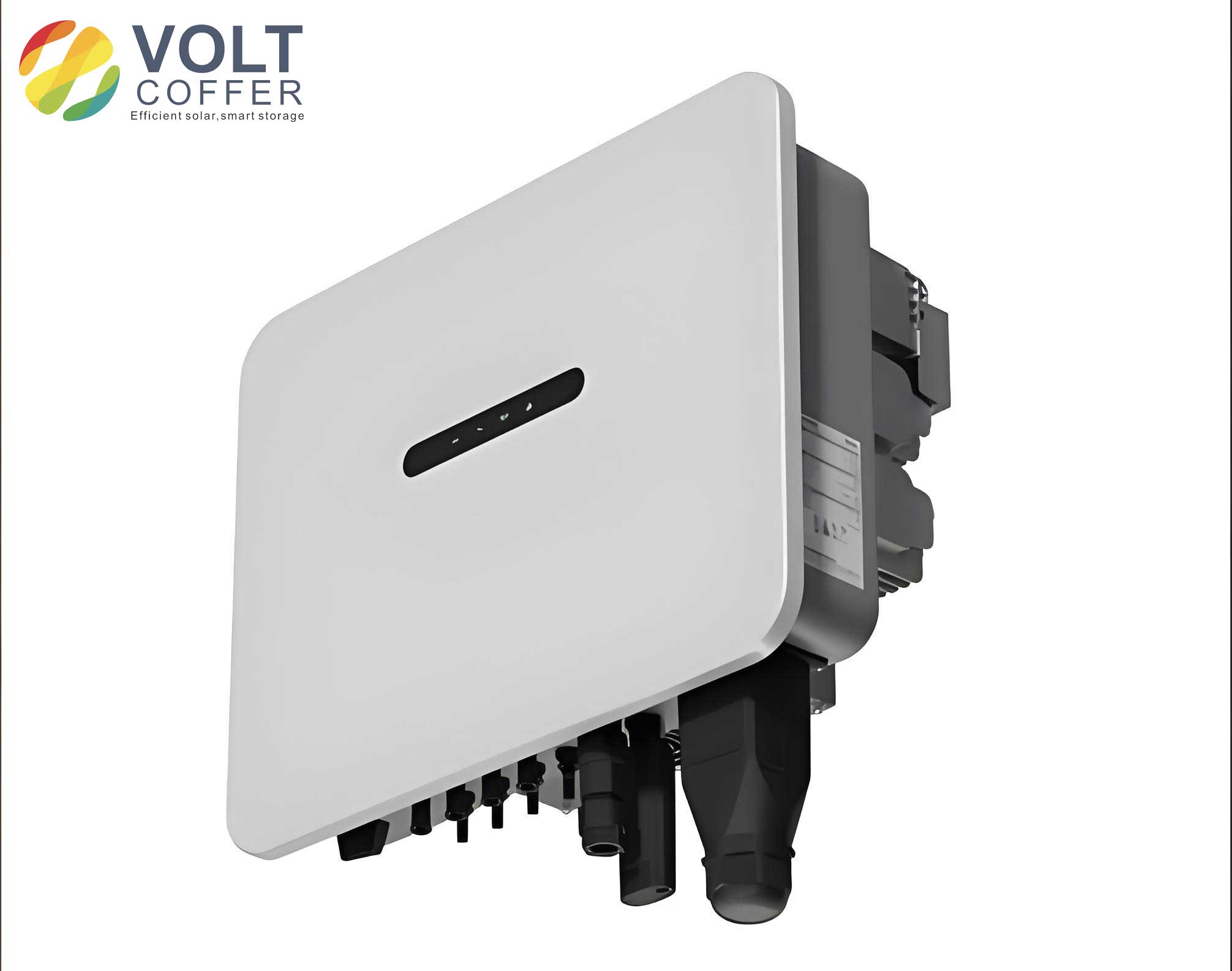
This work investigates a hybrid control paradigm that synergistically combines data-driven learning with foundational control theory to address the nonlinearity in on grid inverter systems. The core idea is to leverage the superior steady-state learning capability of a repetitive controller not for direct control, but as a training mechanism to generate a high-fidelity, trusted dataset of the nonlinear distortion under various operating conditions. This dataset is then processed using an approximate linear regression model to extract a compact, real-time applicable representation of the distortion. Finally, this regressed model is injected as a feedforward compensation signal into a conventional, low-order current controller (e.g., a PI controller). This architecture aims to decouple the goals: the low-order controller ensures robust stability and good dynamic response, while the data-regressed feedforward compensates for the steady-state nonlinear distortion, thereby enhancing the overall performance of the on grid inverter without compromising its stability margins.
Modeling Nonlinear Distortion and Control Loop Analysis
The primary source of nonlinearity in a voltage-source on grid inverter is the inserted dead-time ($T_d$) to prevent shoot-through in the bridge legs. This, along with device voltage drops, introduces a voltage error $V_{DT}(i_x)$ that is a function of the phase current $i_x$ ($x = a, b, c$). For a three-phase system, the average effect over a switching period can be modeled. Under balanced conditions and using a synchronous reference frame ($dq$) transformation with the grid voltage aligned on the d-axis, the nonlinear distortion can be significantly simplified. Assuming $V_{DT}(i_x)$ is an odd function and the commanded d-axis voltage is $V_d^*$, the effective distortion voltage per phase can be approximated as:
$$
V_{DT}(i_x) \approx \frac{3}{4} (V_d^* – R i_x)
$$
where $R$ represents an equivalent resistance. This distortion $V_{DT}$ injects periodic, low-frequency harmonics into the grid current.
The standard method to counteract this is to add a compensation voltage $v_{co}$ to the modulator. Analyzing the control loop reveals crucial insights. The closed-loop transfer function from reference current $i_{ref}$ to inductor current $i_L$ is:
$$
G_{i_{ref}}(s) = \frac{i_L(s)}{i_{ref}(s)} = \frac{G_c(s)G_{pwm}(s)G_p(s)e^{-T_s s}}{1 + G_c(s)G_{pwm}(s)G_p(s)e^{-T_s s}}
$$
where $G_c(s)$ is the current controller, $G_p(s)$ is the plant (filter) transfer function, $G_{pwm}(s)$ is the PWM gain, and $e^{-T_s s}$ models the computational delay. The transfer function from the compensation signal $v_{co}$ to $i_L$ is:
$$
G_{v_{co}}(s) = \frac{i_L(s)}{v_{co}(s)} = \frac{G_{pwm}(s)G_p(s)e^{-T_s s}}{1 + G_c(s)G_{pwm}(s)G_p(s)e^{-T_s s}}
$$
The system’s characteristic equation, governing stability, is $1 + G_c(s)G_{pwm}(s)G_p(s)e^{-T_s s} = 0$. A key observation is that the compensation signal $v_{co}$ can be equivalently applied as $v_{cor} = v_{co}/G_c(s)$ at the reference input. The transfer function for this equivalent path is:
$$
G_{v_{cor}}(s) = \frac{i_L(s)}{v_{cor}(s)} = \frac{G_c(s)G_{pwm}(s)G_p(s)e^{-T_s s}}{1 + G_c(s)G_{pwm}(s)G_p(s)e^{-T_s s}}
$$
While $G_{v_{co}}(s)$ and $G_{v_{cor}}(s)$ are different, they share the same denominator—the system’s characteristic equation. This proves that adding a feedforward compensation signal, whether as $v_{co}$ or $v_{cor}$, does not alter the closed-loop stability of the on grid inverter. This separation principle allows us to design a stabilizing controller ($G_c(s)$) and a compensating feedforward ($v_{cor}$) independently.
Data Generation and Regression Model Development
The proposed methodology involves three distinct stages: data generation and acquisition, data correlation analysis and regression modeling, and final implementation.
Stage 1: Trusted Data Generation via Repetitive Control
To obtain an accurate dataset of the nonlinear distortion, an embedded repetitive controller (RC) is temporarily deployed as an outer loop in the on grid inverter control system. The RC, with its internal model of periodic signals, excels at learning and canceling periodic disturbances like those from dead-time. Once the RC converges in steady-state, the compensation signal it generates ($v_{cor, RC}$) is a high-fidelity representation of the required counter-distortion. This signal, along with synchronous operating point data, is recorded. The operating point vector $\mathbf{x_{in}}$ includes the d-axis reference current $i_{ref}(z)$, DC-link voltage $v_{dc}(z)$, grid voltage $v_g(z)$, and the dead-time $T_d$.
Multiple datasets are collected across different operating points. For each dataset, the periodic compensation signal $v_{cor, RC}$ is decomposed via Fourier analysis to extract the amplitude $A_n$ and phase $\theta_n$ of the fundamental and key low-order harmonics (e.g., 1st, 5th, 7th, 11th, 13th). This forms the core training dataset: $(\mathbf{x_{in}}, A_1, \theta_1, A_5, \theta_5, …)$.
Stage 2: Correlation Analysis and Linear Regression
Before modeling, Pearson correlation analysis is performed to understand the relationship between each input variable in $\mathbf{x_{in}}$ and the output harmonic parameters (amplitudes $A_n$, phases $\theta_n$). The Pearson coefficient $r$ is calculated as:
$$
r = \frac{\sum_{i=1}^{n} (x_i – \bar{x})(y_i – \bar{y})}{\sqrt{\sum_{i=1}^{n} (x_i – \bar{x})^2 \sum_{i=1}^{n} (y_i – \bar{y})^2}}
$$
For the fundamental harmonic amplitude $A_1$, analysis typically shows strong positive correlation with $v_{dc}$ and $T_d$ ($r \approx 0.65-0.66$), and weaker correlation with $i_{ref}$ and $v_g$. For the fundamental phase $\theta_1$, a strong negative correlation with $T_d$ ($r \approx -0.86$) and a significant positive correlation with $i_{ref}$ ($r \approx 0.55$) are observed. This analysis validates which inputs are most influential for modeling each output, guiding the regression process.
A multiple linear regression model is then built for each harmonic parameter ($A_n$, $\theta_n$). The general model is:
$$
\mathbf{Y} = \mathbf{X}\beta + \varepsilon
$$
where $\mathbf{Y}$ is the vector of observed outputs (e.g., all $A_1$ values), $\mathbf{X}$ is the design matrix containing a column of ones (for intercept) and columns for each input variable ($i_{ref}$, $v_{dc}$, $v_g$, $T_d$), $\beta$ is the vector of regression coefficients to be estimated, and $\varepsilon$ is the error vector.
The ordinary least squares (OLS) estimate $\hat{\beta}$ minimizes the sum of squared residuals $E_i$:
$$
\min E_i = \sum_{i=1}^{n} (y_i – \hat{y}_i)^2 = (\mathbf{Y} – \mathbf{X}\hat{\beta})'(\mathbf{Y} – \mathbf{X}\hat{\beta})
$$
Solving $\partial E_i / \partial \hat{\beta} = 0$ yields the optimal coefficient vector:
$$
\hat{\beta} = (\mathbf{X}’\mathbf{X})^{-1}\mathbf{X}’\mathbf{Y}
$$
To compare the influence of different input variables (which have different units), standardized regression coefficients $\hat{\beta}^*$ are computed:
$$
\hat{\beta}^*_i = \hat{\beta}_i \frac{s_i}{s_y}
$$
where $s_i$ and $s_y$ are the standard deviations of the $i$-th predictor and the response variable, respectively.
The quality and statistical significance of each regression model is assessed. The total sum of squares (SST) is partitioned into the regression sum of squares (SSR) and the error sum of squares (SSE): $SST = SSR + SSE$. The coefficient of determination $R^2 = SSR/SST$ indicates the proportion of variance explained by the model. An F-test is performed where $F = MSR / MSE$ with $MSR = SSR/p$ and $MSE = SSE/(n-p-1)$, testing the null hypothesis that all regression coefficients are zero. A low p-value ($p < 0.01$) and an $R^2$ close to 1 indicate a good fit.
For example, the regression results for the fundamental harmonic amplitude $A_1$ might be as follows:
| Parameter | $\hat{\beta}_{1,amp}$ | $\hat{\beta}^{*}_{1,amp}$ |
|---|---|---|
| Constant | -0.4145 | – |
| $i_{ref}(z)$ | 0.0616 | 0.4898 |
| $v_{dc}(z)$ | 0.0016 | 0.5986 |
| $v_g(z)$ | 0.0023 | 0.1928 |
| $T_d$ | 0.1436 | 0.6197 |
And its associated ANOVA table:
| Source | SS | df | MS | F | p-value |
|---|---|---|---|---|---|
| Regression (SSR) | 2.041 | 4 | 0.510 | 1791.4 | 0.000 |
| Residual (SSE) | 0.026 | 91 | 0.000285 | ||
| Total (SST) | 2.066 | 95 | – | – | – |
This shows a high $R^2 \approx 0.987$ and a highly significant F-statistic, confirming the model’s validity. Similar models are built for $\theta_1$, $A_5$, $\theta_5$, etc. The L2-norm loss for the fundamental amplitude model, $L_2 = \frac{1}{n}\sum (y_i – \hat{y}_i)^2$, would be very small (e.g., 0.016), indicating high accuracy.
Stage 3: Real-Time Compensation Implementation
With all regression models $\hat{\beta}_n$ for amplitudes and phases, the final compensation signal for the on grid inverter is synthesized in real-time. For any given operating point $\mathbf{x_{in}}$, the amplitude and phase for each harmonic $n$ are calculated instantly:
$$
\begin{aligned}
\hat{A}_n &= \beta_{n,amp,0} + \beta_{n,amp,1} \cdot i_{ref} + \beta_{n,amp,2} \cdot v_{dc} + \beta_{n,amp,3} \cdot v_g + \beta_{n,amp,4} \cdot T_d \\
\hat{\theta}_n &= \beta_{n,theta,0} + \beta_{n,theta,1} \cdot i_{ref} + \beta_{n,theta,2} \cdot v_{dc} + \beta_{n,theta,3} \cdot v_g + \beta_{n,theta,4} \cdot T_d
\end{aligned}
$$
The total compensation current $i_{com}$ is then constructed in the stationary $\alpha\beta$ frame:
$$
i_{com} = \sum_{n \in \{1,5,7,11,13\}} \hat{A}_n \sin(n \omega t + \hat{\theta}_n)
$$
This signal $i_{com}$ is directly added to the output of the primary current controller (e.g., a PI controller) as the feedforward term $v_{cor}$. This architecture leverages the robustness and fast dynamics of the simple PI controller while using the data-regressed model to cancel the steady-state nonlinear distortion. The process significantly reduces the memory footprint compared to a full LUT-based approach and avoids the dynamic limitations of an embedded repetitive controller, creating a high-performance on grid inverter control system.
Experimental Validation and Performance Analysis
The proposed data-regression compensation method was validated on a three-phase two-level on grid inverter prototype. Key parameters were: switching frequency $f_s = 10$ kHz, filter inductance $L = 3.8$ mH, DC-link voltage $V_{dc} = 400$ V, and grid phase voltage $V_g = 150$ V.
First, the performance of the traditional repetitive controller (RC) was evaluated. Without any compensation, the grid current exhibited severe zero-crossing distortion. Upon activating the RC, this distortion was eliminated, and current quality improved markedly, demonstrating RC’s effectiveness as a steady-state learner and data generator. The compensation signals $i_{com,\alpha}$ and $i_{com,\beta}$ generated by the RC were recorded for dataset creation. However, as anticipated, the RC showed poor dynamic response. During a step change in reference current amplitude from 5 A to 10 A, the output current exhibited pronounced oscillatory behavior lasting for several grid cycles before settling.
Second, the proposed regression-based feedforward compensator was tested. In steady-state, its performance was nearly identical to the RC: it effectively suppressed the zero-crossing distortion and produced a clean sinusoidal current. The shape and magnitude of the generated $i_{com,\alpha}$ and $i_{com,\beta}$ were very similar to those from the RC, confirming the accuracy of the regression model. Crucially, during the same dynamic step change (5 A to 10 A), the system with the regression compensator showed a fast, well-damped response. No significant overshoot or oscillatory settling was observed, highlighting the superior dynamic performance achieved by pairing the static regression model with a low-bandwidth PI controller, compared to the inherently slow dynamics of the embedded RC. This validates the core advantage of the proposed architecture for the on grid inverter: high steady-state accuracy without sacrificing dynamic response.
Conclusion
This work presents a pragmatic and effective method for compensating nonlinear characteristics in grid-connected inverters by fusing data-driven learning with classical control principles. The method systematically addresses key challenges in applied data-driven control: data provenance (using RC as a trusted trainer), model realizability (using lightweight linear regression), and stable integration (using feedforward injection that doesn’t affect closed-loop stability). The resulting compensator requires minimal memory, imposes negligible real-time computational burden, and seamlessly integrates with standard current controllers. Experimental results on a three-phase on grid inverter demonstrate that the approach achieves compensation performance rivaling that of a repetitive controller in steady-state, while simultaneously offering significantly improved dynamic response. This “small-data” regression enhanced control strategy provides a viable and high-performance engineering solution for improving the power quality of on grid inverter systems affected by dead-time and similar nonlinearities.