
The global pursuit of sustainable energy has dramatically transformed the energy landscape over the past few decades. Among various renewable sources, the development and integration of solar panels have been particularly remarkable. From virtually negligible contributions at the turn of the century, solar energy has grown to account for a significant and rapidly expanding share of global power generation. This growth is fueled by the inherent advantages of solar power: it is clean, abundant, and offers a critical pathway to mitigating global energy shortages and combating climate change. Maximizing the efficiency of solar panels is therefore a paramount objective in both research and practical engineering. Numerous studies have identified a wide array of factors influencing the final power output of a photovoltaic (PV) system. These factors range from the intrinsic properties of the solar panels themselves, such as the semiconductor materials and manufacturing processes, to external environmental conditions like solar irradiance and temperature, and further to system-level components including the efficiency of inverters, wiring, and the configuration of the PV array.
This analysis focuses on one of the most critical and readily adjustable parameters in fixed-tilt photovoltaic installations: the tilt angle of the solar panels. The angle at which a panel is inclined relative to the horizontal plane directly determines the amount of solar radiation it intercepts over the course of a day and a year. By optimizing this angle, we can significantly enhance the energy yield of a PV system without increasing the number of solar panels. This study involves a detailed computational analysis to determine the optimal fixed tilt angle for a specific project location, calculating the resultant energy generation and projecting performance over the system’s lifetime.
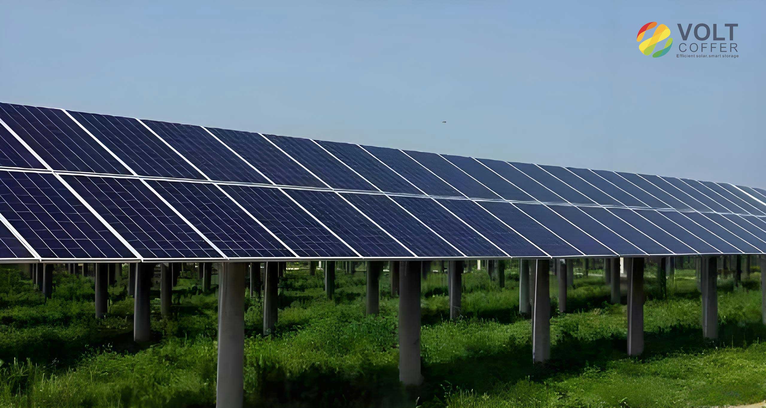
The project site is characterized by a continental cold-temperate climate. The key climatic features include arid springs with frequent winds, brief summers and autumns, and prolonged, severely cold winters with extreme temperature variations. Summer peak temperatures can reach 38.7°C, while winter lows can plummet to -51.5°C, with an annual average of approximately 1.9°C. The region experiences about 90 days per year with minimum temperatures below -20°C. Annual precipitation is low, averaging 158.3 mm, contrasted by a high evaporation rate of 1,734 mm. The area benefits from substantial sunshine, with an average of 2,869.8 hours of annual sunlight. The frost-free period in primary agricultural zones averages 108 days. Common meteorological hazards include cold waves, blizzards in winter, and droughts, dry hot winds, and hail in other seasons.
From a solar resource perspective, the site is exceptionally well-suited for photovoltaic projects. The annual average solar radiation total is 5,407 MJ/m² on a horizontal surface. According to the Chinese Meteorological Industry Standard QX/T89-2008, which classifies solar resource richness based on annual total radiation, this level falls into the “very abundant” category. Solar radiation follows a predictable monthly pattern, peaking in the summer months (June-July) and reaching a minimum in winter. Radiation increases from January to June and decreases from July to December. The proposed installation utilizes a large array of solar panels, with each module having dimensions of 1,650 mm by 992 mm. The total number of modules is 126,000, leading to a combined installed capacity of 30,240 kW (or 30.24 MW).
Methodology for Power and Performance Calculation
The annual energy yield of a grid-connected photovoltaic system can be estimated using a fundamental formula that considers the installed capacity, available solar energy, and overall system efficiency. The calculation is expressed as:
$$ L = W \times H \times \eta \times 0.1 $$
Where:
\( L \) is the annual energy generation (in 10,000 kWh).
\( W \) is the total installed capacity (in 10,000 kW).
\( H \) is the annual peak sun hours (in hours), which is equivalent to the annual in-plane irradiation (in kWh/m²) divided by the standard irradiance of 1 kW/m².
\( \eta \) is the total efficiency of the grid-connected PV system, accounting for losses in solar panels, wiring, inverters, and other components.
The factor 0.1 is used for unit conversion within this specific formulation.
Evaluating the long-term performance of solar panels requires an understanding of their degradation. The power degradation rate is a standard metric defined by comparing the maximum output power at the beginning of operation to the power measured after a period of time, typically one year and beyond. The degradation rate (\( DR \)) is calculated as follows:
$$ DR = \frac{P_{\text{max, initial}} – P_{\text{max, after time t}}}{P_{\text{max, initial}}} \times 100\% $$
Where \( P_{\text{max, initial}} \) is the initial maximum output power measured under standard test conditions (STC) and \( P_{\text{max, after time t}} \) is the maximum output power measured after the system has been operational for a specified duration under real-world conditions.
Determining the Optimal Tilt Angle for Solar Panels
The geographic coordinates for the project site are approximately 46°53′ North latitude and 89°40′ East longitude. To find the optimal fixed tilt angle, we employ a solar radiation model that accounts for the anisotropic nature of the sky (the Klein and Theilacker model is a common reference). This model allows us to translate the known long-term average monthly global horizontal irradiance (GHI) into the total in-plane irradiance (POA) received by the surface of the solar panels at various tilt angles. The objective is to find the angle that maximizes the annual cumulative POA irradiation.
The results of this calculation for tilt angles ranging from 30° to 40° are summarized in the table below. The monthly and annual total radiation values (in MJ/m²) are presented for each angle.
| Month | 30° | 31° | 32° | 33° | 34° | 35° | 36° | 37° | 38° | 39° | 40° |
|---|---|---|---|---|---|---|---|---|---|---|---|
| January | 274 | 276 | 278 | 280 | 281 | 283 | 285 | 286 | 288 | 289 | 290 |
| February | 466 | 469 | 472 | 476 | 479 | 482 | 485 | 488 | 490 | 493 | 496 |
| March | 533 | 534 | 535 | 537 | 538 | 539 | 540 | 541 | 541 | 542 | 542 |
| April | 613 | 613 | 613 | 612 | 612 | 611 | 610 | 609 | 608 | 607 | 605 |
| May | 687 | 685 | 683 | 680 | 678 | 675 | 672 | 670 | 667 | 663 | 660 |
| June | 689 | 686 | 683 | 680 | 677 | 673 | 670 | 666 | 662 | 658 | 654 |
| July | 673 | 671 | 668 | 665 | 662 | 659 | 656 | 653 | 650 | 646 | 642 |
| August | 637 | 637 | 636 | 635 | 633 | 632 | 631 | 629 | 627 | 625 | 623 |
| September | 580 | 581 | 583 | 584 | 585 | 586 | 587 | 588 | 588 | 589 | 589 |
| October | 444 | 447 | 449 | 452 | 455 | 458 | 460 | 462 | 464 | 467 | 469 |
| November | 329 | 332 | 336 | 339 | 342 | 345 | 348 | 351 | 353 | 356 | 359 |
| December | 273 | 276 | 279 | 282 | 285 | 288 | 291 | 294 | 297 | 299 | 302 |
| Annual Total | 6,198 | 6,207 | 6,215 | 6,222 | 6,227 | 6,231 | 6,235 | 6,237 | 6,235 | 6,234 | 6,231 |
Analysis of the table reveals a clear maximum. The annual total in-plane radiation peaks at 6,237 MJ/m² for a tilt angle of 37°. This represents a significant 15.6% increase compared to the horizontal plane radiation of 5,395 MJ/m². The data shows that the optimal angle is quite pronounced; moving away from 37° in either direction results in a lower annual energy yield. The monthly distribution also shifts with the tilt angle. For lower angles (30°, 31°), maximum monthly radiation occurs in June, while for the optimal and higher angles, the peak shifts to May. This is because a steeper tilt angle is better aligned with the lower sun path in winter, capturing more energy in the shoulder seasons, albeit at the expense of slightly reducing summer capture when the sun is high. Critically, for the optimal 37° tilt, the months from April to September collectively receive over 62% of the annual radiation, defining the prime generation period for the solar panels. Consequently, this tilt angle of 37° is selected as the optimal fixed installation angle for the photovoltaic array at this site.
First-Year Energy Generation Statistics
Using the optimal tilt angle and applying the power generation formula with appropriate system efficiency factors, the first year of operational energy production can be calculated. The relationship between radiation and electrical energy output is governed by the system’s performance, often simplified by a conversion factor. For this analysis, the effective conversion is taken as approximately 1.526 MJ/m² per kWh of generation for calculation purposes. The monthly and annual energy yield for the inaugural year are presented below.
| Month | In-Plane Radiation at 37° (MJ/m²) | Monthly Energy Generation (10,000 kWh) |
|---|---|---|
| January | 286 | 187 |
| February | 488 | 320 |
| March | 541 | 355 |
| April | 609 | 399 |
| May | 670 | 439 |
| June | 666 | 436 |
| July | 653 | 428 |
| August | 629 | 412 |
| September | 588 | 385 |
| October | 462 | 303 |
| November | 351 | 230 |
| December | 294 | 193 |
| Annual Total | 6,236 | 4,087 |
The total first-year energy generation from the array of solar panels was 40.87 million kWh. The monthly generation profile follows a parabolic trend, closely mirroring the solar resource. Generation rises from a winter low of 1.87 million kWh in January to a peak of 4.39 million kWh in May. Interestingly, output in June (4.36 million kWh) is slightly lower than in May, which can typically be attributed to local weather patterns such as increased cloud cover or precipitation during that month, demonstrating how real-world conditions can cause deviations from the idealized solar radiation curve.
Long-Term Energy Yield Forecast Over 25 Years
The performance of photovoltaic modules degrades slowly over time. It is standard practice to model and guarantee energy production over a long-term period, typically 25 years. The initial STC-rated annual energy output was calculated at 41.28 million kWh. The actual first-year output was 40.87 million kWh. Applying the degradation rate formula, the first-year degradation is calculated as:
$$ DR_{\text{Year 1}} = \frac{41.28 – 40.87}{41.28} \times 100\% \approx 1.0\% $$
Standard industry projection models, such as those implemented in PV simulation software (e.g., PVsyst), are used to forecast future output. A common degradation profile assumes a higher initial degradation rate, stabilizing at a lower rate later in the system’s life. For this projection, we assume an annual degradation of approximately 1.0% for the first 10 years, followed by a reduced rate of about 0.67% per year for years 11 through 25. The forecasted annual energy generation for the 25-year period is detailed in the following table.
| Year of Operation | Annual Energy (10,000 kWh) | Year of Operation | Annual Energy (10,000 kWh) |
|---|---|---|---|
| First Year | 4,087 | 14th Year | 3,634 |
| 2nd Year | 4,046 | 15th Year | 3,610 |
| 3rd Year | 4,006 | 16th Year | 3,586 |
| 4th Year | 3,965 | 17th Year | 3,562 |
| 5th Year | 3,926 | 18th Year | 3,538 |
| 6th Year | 3,887 | 19th Year | 3,514 |
| 7th Year | 3,848 | 20th Year | 3,491 |
| 8th Year | 3,809 | 21st Year | 3,467 |
| 9th Year | 3,771 | 22nd Year | 3,444 |
| 10th Year | 3,733 | 23rd Year | 3,421 |
| 11th Year | 3,708 | 24th Year | 3,398 |
| 12th Year | 3,684 | 25th Year | 3,375 |
| 13th Year | 3,659 | 25-Year Cumulative Total | 92,169 |
| 25-Year Average (Annual) | 3,687 | ||
The long-term forecast indicates robust performance from the installation of solar panels. Over the 25-year operational period, the system is projected to generate a cumulative total of 921.69 million kWh of clean electricity. The average annual generation over this period is forecasted to be 36.87 million kWh. By the end of the 25th year, the system’s energy output is expected to have degraded to approximately 3.375 million kWh. The cumulative degradation rate at the end of the period can be expressed relative to the first-year actual output:
$$ DR_{\text{Year 25}} = \frac{4,087 – 3,375}{4,087} \times 100\% \approx 17.4\% $$
This aligns with typical performance warranties for high-quality solar panels, which often guarantee at least 80-82% of the original power output after 25 years.
Conclusion
This comprehensive analysis underscores the critical importance of optimizing the tilt angle for fixed-tilt photovoltaic installations. For the specific high-latitude, cold-climate project site, computational modeling of solar radiation incidence revealed that an inclination of 37° maximizes the annual energy harvest. At this optimal angle, the surface of the solar panels receives 6,237 MJ/m² per year, a 15.6% increase over horizontal placement. This directly translates to maximized system efficiency and improved economic returns. The first year of operation validated the model, yielding 40.87 million kWh with a generation profile that peaked in late spring. Long-term performance projections, accounting for standard photovoltaic degradation rates, forecast a cumulative generation of 921.69 million kWh over 25 years, with an average annual output of 36.87 million kWh and a terminal degradation of approximately 17.4%. This case study demonstrates that meticulous site-specific engineering, starting with the fundamental optimization of the solar panels‘ orientation, is essential for unlocking the full potential of solar energy resources and ensuring the long-term viability and productivity of photovoltaic power plants.