
As a renewable energy source, solar power is widely recognized as a pivotal solution for optimizing the global energy structure and mitigating climate change. Among various photovoltaic technologies, thin film solar panels have emerged as a promising third-generation approach due to their cost-effectiveness, flexibility, lightweight nature, and potential for large-scale deployment. In this article, I will delve into the fundamental working principles, classification, and performance characterization of thin film solar panels, with a particular emphasis on the application of electrochemical impedance spectroscopy (EIS) for analyzing internal charge transport and transfer processes. Through detailed discussions and illustrative examples, I aim to provide a comprehensive understanding of how advanced characterization techniques can guide the development of high-efficiency thin film solar panels.
The transition from fossil fuels to sustainable energy systems necessitates innovations in solar technology. Traditional crystalline silicon solar cells, while dominant, face limitations such as high material consumption, rigidity, and energy-intensive manufacturing. Thin film solar panels address these challenges by utilizing thinner active layers (typically micrometers in thickness) deposited on flexible substrates like plastic, metal foils, or glass. This not only reduces material usage but also enables novel applications in building-integrated photovoltaics, portable electronics, and aerospace. The core mechanism of thin film solar panels involves the photovoltaic effect: when photons strike a semiconductor material, electron-hole pairs are generated, and their separation at a p-n junction or similar interface produces an electric current. The efficiency of this process depends on factors such as light absorption, charge carrier mobility, and recombination losses, which vary across different thin film technologies.
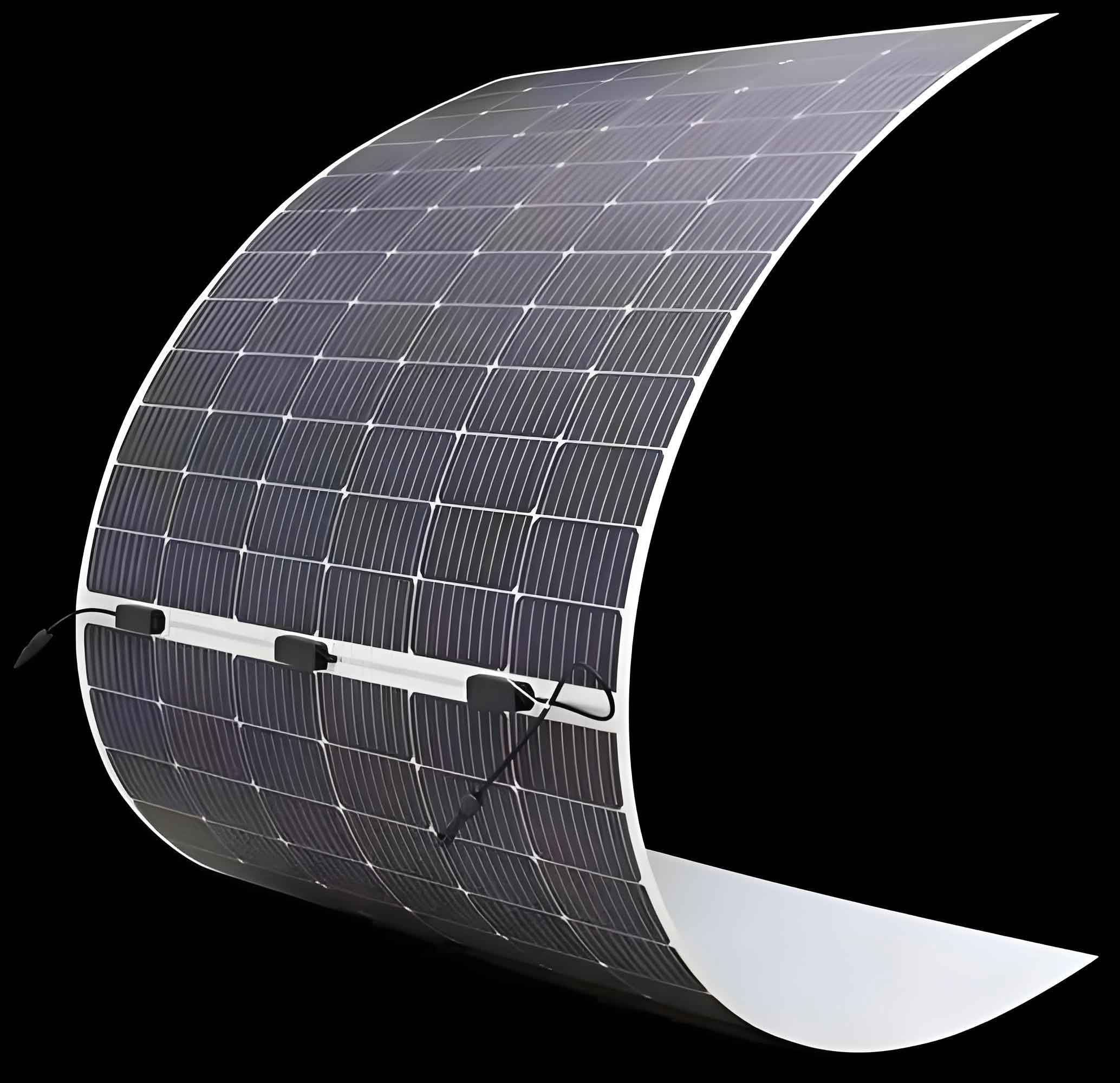
To categorize thin film solar panels, I will outline four major types based on their active materials: amorphous silicon (a-Si), copper indium gallium selenide (CIGS), organic photovoltaics (OPV), and dye-sensitized solar cells (DSSC). Each type has distinct properties, fabrication methods, and challenges, as summarized in the table below. The development of thin film solar panels often involves trade-offs between efficiency, stability, and cost, necessitating tailored characterization strategies to optimize performance.
| Type of Thin Film Solar Panel | Typical Materials | Bandgap Range (eV) | Advantages | Challenges | Common Deposition Methods |
|---|---|---|---|---|---|
| Amorphous Silicon (a-Si) | Hydrogenated non-crystalline silicon | 1.7–1.8 | High absorption coefficient, low-temperature processing, flexibility | Light-induced degradation (Staebler-Wronski effect), moderate efficiency | Plasma-enhanced chemical vapor deposition (PECVD) |
| Copper Indium Gallium Selenide (CIGS) | Cu(In,Ga)Se2 or related compounds | 1.0–1.7 (tunable) | High efficiency, good stability, tolerance to defects | High deposition temperature, scarcity of indium, complex stoichiometry | Sputtering, co-evaporation, solution processing |
| Organic Photovoltaics (OPV) | Polymer donors (e.g., P3HT) and acceptors (e.g., PCBM) | 1.5–2.2 | Ultra-flexibility, lightweight, low-cost roll-to-roll fabrication | Low stability under environmental stress, limited efficiency | Spin-coating, inkjet printing, slot-die coating |
| Dye-Sensitized Solar Cells (DSSC) | Organic dyes on mesoporous TiO2 with electrolyte | 1.5–2.0 (dye-dependent) | Low-cost materials, vibrant colors, works under diffuse light | Liquid electrolyte leakage, durability issues, moderate efficiency | Screen printing, doctor blading, electrochemical deposition |
Beyond these traditional types, perovskite solar cells have recently gained prominence as a high-efficiency variant of thin film solar panels. With a general formula of ABX3 (e.g., CH3NH3PbI3), perovskite materials exhibit exceptional light absorption, long carrier diffusion lengths, and tunable bandgaps. A typical perovskite thin film solar panel consists of multiple layers: a transparent conductive oxide (TCO) substrate, an electron transport layer (ETL, e.g., TiO2 or SnO2), a perovskite active layer, a hole transport layer (HTL, e.g., spiro-OMeTAD), and a metal back electrode. The performance of such thin film solar panels is governed by interfacial charge transfer and bulk recombination, which can be probed using advanced electrochemical techniques.
Characterizing thin film solar panels involves evaluating key performance parameters derived from current-density-voltage (J-V) measurements under standard test conditions (AM 1.5G illumination, 100 mW/cm2). The primary metrics include:
- Short-circuit current density (Jsc): The maximum current output per unit area when the voltage is zero, expressed in mA/cm2. It depends on the light absorption and charge collection efficiency of the thin film solar panel.
- Open-circuit voltage (Voc): The voltage at zero current, determined by the quasi-Fermi level splitting in the active layer. For an ideal thin film solar panel, Voc relates to the bandgap and recombination losses.
- Fill factor (FF): A measure of the “squareness” of the J-V curve, defined as the ratio of maximum power output to the product of Jsc and Voc:
$$ FF = \frac{P_{max}}{J_{sc} \times V_{oc}} = \frac{J_{mp} \times V_{mp}}{J_{sc} \times V_{oc}} $$
where Jmp and Vmp are the current density and voltage at the maximum power point. - Power conversion efficiency (PCE): The ultimate figure of merit, calculated as:
$$ PCE = \frac{P_{max}}{P_{in}} = \frac{J_{sc} \times V_{oc} \times FF}{P_{in}} $$
with Pin being the incident light power (typically 100 mW/cm2). - Incident photon-to-current efficiency (IPCE): Also known as external quantum efficiency (EQE), it quantifies the spectral response of a thin film solar panel at specific wavelengths:
$$ IPCE(\lambda) = \frac{1240 \times J_{sc}(\lambda)}{\lambda \times P_{in}(\lambda)} \times 100\% $$
where λ is the wavelength in nanometers.
These parameters provide a macroscopic overview, but to understand the underlying dynamics—such as charge transport, recombination, and interfacial kinetics—electrochemical impedance spectroscopy (EIS) is indispensable.
Electrochemical impedance spectroscopy is a non-destructive technique that applies a small sinusoidal voltage or current perturbation across a wide frequency range (typically mHz to MHz) to a thin film solar panel and measures the system’s response. The impedance Z(ω) is a complex function defined as:
$$ Z(\omega) = \frac{V(\omega)}{I(\omega)} = Z’ + jZ” $$
where ω = 2πf is the angular frequency, Z’ is the real part (resistive component), Z” is the imaginary part (reactive component), and j is the imaginary unit. For thin film solar panels, EIS data can be modeled using equivalent circuits composed of resistors, capacitors, and constant phase elements (CPEs) that represent physical processes. A common equivalent circuit for a typical thin film solar panel, such as a perovskite device, includes:
- Series resistance (Rs): Accounts for ohmic losses from contacts and electrodes.
- Charge transfer resistance (Rct): Represents the resistance to charge transfer at interfaces, e.g., between the perovskite layer and the transport layers.
- Chemical capacitance (Cμ): Associated with the density of states in the active layer, reflecting carrier accumulation.
- Recombination resistance (Rrec): Correlates with bulk or interfacial recombination processes.
- Constant phase element (CPE): Often used instead of an ideal capacitor to account for non-ideal behavior due to surface roughness or heterogeneity in thin film solar panels.
The impedance of a simplified Randles circuit, often applicable to thin film solar panels, is given by:
$$ Z(\omega) = R_s + \frac{R_{ct}}{1 + (j\omega R_{ct} C_{dl})^\alpha} $$
where Cdl is the double-layer capacitance and α is the CPE exponent (0 ≤ α ≤ 1). EIS data are typically presented in two forms:
- Nyquist plot: A plot of -Z” versus Z’, where semicircles correspond to different time constants. For instance, a high-frequency semicircle may represent charge transfer at the ETL/perovskite interface, while a low-frequency arc relates to ion migration or recombination in thin film solar panels.
- Bode plot: Consists of two graphs—|Z| versus frequency and phase angle (θ) versus frequency. The Bode plot helps identify characteristic frequencies and time constants of processes within the thin film solar panel.
To illustrate the utility of EIS, I analyzed a case study on perovskite thin film solar panels with varying compositional gradients (e.g., different halide ratios, denoted as x in mixed-halide perovskites). By fitting EIS spectra measured under different bias voltages, I extracted parameters like Rct and Cμ to compute the electron lifetime (τn), a critical indicator of recombination:
$$ \tau_n = R_{rec} \times C_{\mu} $$
This electron lifetime reflects how long photogenerated carriers survive before recombining. For example, in a perovskite thin film solar panel with x=0.2 composition, τn was found to be higher at biases above 0.4 V, suggesting suppressed recombination compared to other formulations. However, at lower biases, the chemical capacitance changes due to shifts in the Fermi level of the TiO2 electron transport layer, complicating direct comparisons. Such insights underscore how EIS can decode the intricate charge dynamics in thin film solar panels, guiding material optimization.
To further elucidate the performance variations among thin film solar panels, I have compiled a table summarizing typical EIS-derived parameters for different technologies under one-sun illumination. These values are illustrative and can vary based on fabrication conditions and device architecture.
| Thin Film Solar Panel Type | Series Resistance Rs (Ω·cm2) | Charge Transfer Resistance Rct (Ω·cm2) | Chemical Capacitance Cμ (F/cm2) | Electron Lifetime τn (ms) | Dominant Recombination Pathway |
|---|---|---|---|---|---|
| Amorphous Silicon (a-Si) | 5–15 | 50–200 | 10-6–10-5 | 0.1–1 | Defect-assisted Shockley-Read-Hall recombination |
| CIGS | 1–10 | 100–500 | 10-5–10-4 | 1–10 | Interface recombination at buffer/absorber junction |
| Organic (OPV) | 10–50 | 200–1000 | 10-7–10-6 | 0.01–0.1 | Geminate and non-geminate recombination in bulk heterojunction |
| Dye-Sensitized (DSSC) | 5–20 | 20–100 (for redox electrolyte) | 10-4–10-3 | 1–100 | Charge recombination at TiO2/dye/electrolyte interface |
| Perovskite (e.g., MAPbI3) | 2–10 | 100–1000 | 10-4–10-3 | 0.1–10 | Ionic migration and trap-assisted recombination |
The analysis of thin film solar panels via EIS is not without limitations. While it offers quantitative insights into charge transfer and recombination, it cannot directly pinpoint the atomic-scale origins of defects or the exact nature of recombination centers. Therefore, complementary techniques are often employed alongside EIS to build a holistic understanding. For instance, transient photovoltage (TPV) and transient photocurrent (TPC) measurements probe carrier dynamics on micro- to millisecond timescales. Photoluminescence (PL) and electroluminescence (EL) spectroscopy reveal radiative recombination and trap states. Additionally, space-charge-limited current (SCLC) measurements quantify trap densities in the active layers of thin film solar panels. Integrating these methods with EIS allows researchers to correlate macroscopic impedance responses with microscopic material properties.
Looking ahead, the future of thin film solar panels hinges on overcoming key challenges such as long-term stability, scalability, and environmental sustainability. For perovskite thin film solar panels, issues like ion migration, moisture sensitivity, and lead toxicity require urgent attention. Advanced encapsulation techniques and lead-free alternatives (e.g., tin-based perovskites) are being actively explored. Moreover, tandem architectures that combine multiple thin film solar panels—such as perovskite-on-silicon or all-perovskite stacks—promise to surpass the Shockley-Queisser efficiency limit. In all these endeavors, characterization tools like EIS will remain vital for diagnosing performance bottlenecks and accelerating innovation.
In conclusion, thin film solar panels represent a versatile and evolving class of photovoltaic devices with immense potential to reshape the energy landscape. Through detailed characterization using current-voltage metrics and electrochemical impedance spectroscopy, we can unravel the complex charge transport and transfer processes that govern their efficiency. While EIS provides powerful macroscopic insights, coupling it with other spectroscopic and electrical techniques will enable a deeper dive into defect physics and interfacial engineering. As research progresses, the continued refinement of thin film solar panels—driven by interdisciplinary collaboration and advanced characterization—will pave the way for affordable, durable, and high-performance solar energy solutions.