
The accurate and reliable management of energy storage systems is paramount in modern applications ranging from electric vehicles to grid-scale storage. At the heart of these systems lies the li ion battery, prized for its high energy density and longevity. To ensure the safety, efficiency, and longevity of a li ion battery pack, a sophisticated Battery Management System (BMS) is indispensable. The BMS continuously monitors operational parameters like voltage, current, and temperature, and, more critically, estimates internal states that cannot be measured directly. Among these, the State of Charge (SOC)—defined as the ratio of remaining charge to the maximum available charge—is arguably the most crucial parameter. It is the electrochemical equivalent of a fuel gauge, informing users and control systems about the instantaneous available energy. Precise SOC knowledge prevents harmful operating conditions such as overcharge and deep discharge, which accelerate the aging of a li ion battery. However, SOC cannot be measured by a simple sensor; it must be inferred or estimated through algorithms based on measurable signals like current and voltage.
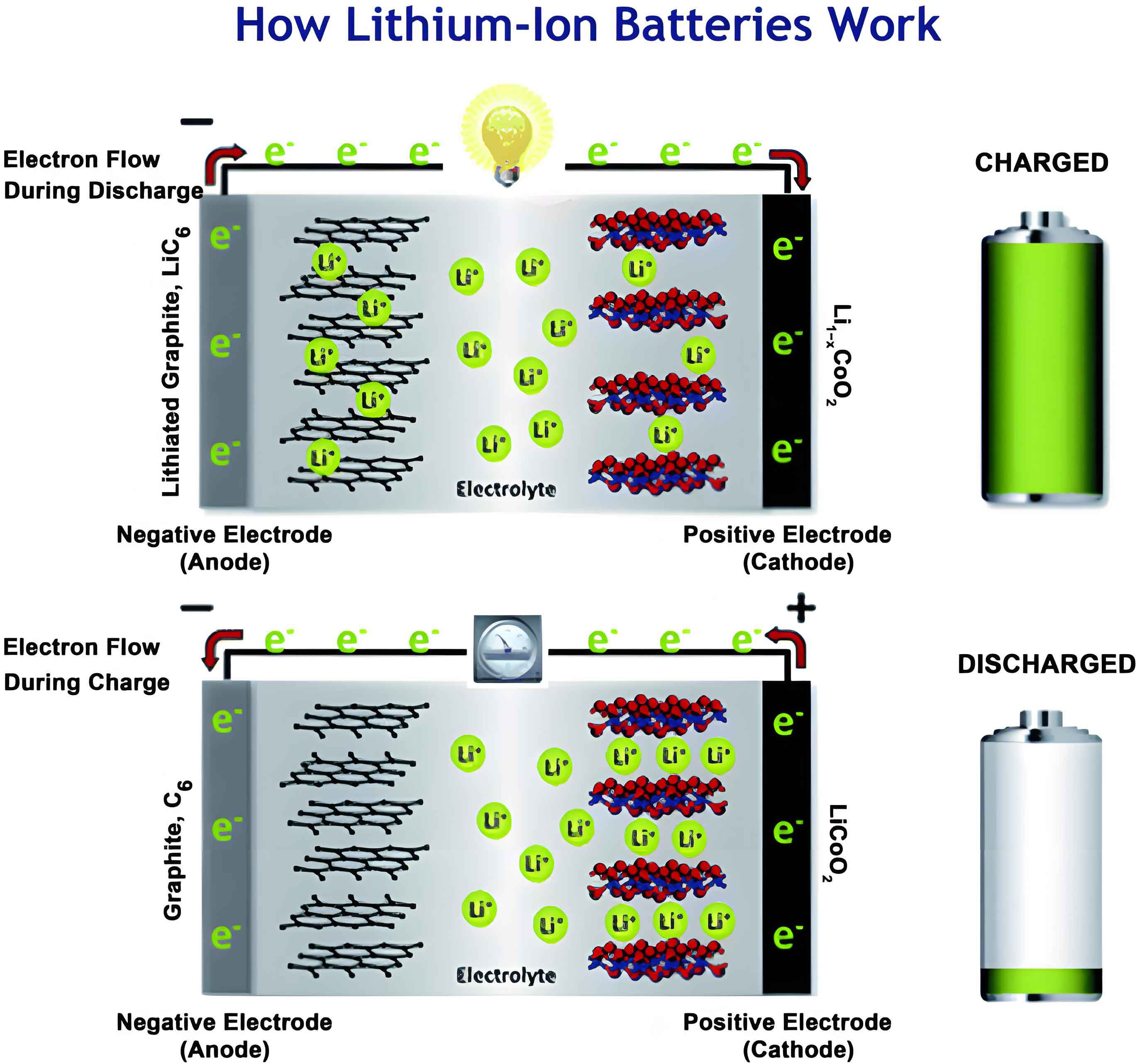
The quest for accurate SOC estimation for the li ion battery has led to numerous methodologies, broadly categorized into offline and online techniques. Online methods, suitable for real-time BMS operation, include Coulomb Counting, data-driven approaches, and model-based filters. Coulomb Counting is simple but suffers from error accumulation due to sensor inaccuracies and an unknown initial SOC. Data-driven methods, such as those employing neural networks, can achieve high accuracy but require extensive training data and computational resources. Model-based filters strike a balance, offering reasonable accuracy with manageable computational complexity. These filters use a mathematical model of the li ion battery—often an Equivalent Circuit Model (ECM)—and a recursive algorithm to optimally combine model predictions with real-time measurements. The Kalman Filter (KF) and its nonlinear variants, such as the Extended Kalman Filter (EKF), Unscented Kalman Filter (UKF), and Cubature Kalman Filter (CKF), have become prominent in this domain. The CKF, in particular, offers a derivative-free solution with good numerical stability and accuracy for Gaussian noise by using a third-degree spherical-radial cubature rule. However, the standard CKF’s performance can degrade when the underlying li ion battery model is inaccurate or when the system experiences abrupt changes or persistent disturbances, leading to filter divergence.
This work addresses this robustness challenge by proposing an enhanced algorithm: the Adaptive Fading Cubature Kalman Filter (AFCKF). The core innovation is the integration of an adaptive fading factor into the CKF framework. This factor automatically adjusts based on the discrepancy between theoretical and actual innovation sequences, effectively “forgetting” past data at a controlled rate when a model mismatch is detected. This mechanism suppresses filter divergence and maintains estimation stability. The subsequent sections detail the development of a second-order ECM for the li ion battery, the theoretical derivation of the AFCKF algorithm, and a comprehensive simulation-based validation comparing its performance against the standard CKF and an Adaptive CKF (ACKF) on two distinct li ion battery types.
Mathematical Modeling of the Li-Ion Battery
An accurate yet computationally tractable model is the foundation for any model-based estimation algorithm. For SOC estimation of a li ion battery, Equivalent Circuit Models (ECMs) are widely adopted. They use electrical components like resistors, capacitors, and voltage sources to mimic the dynamic behavior of the electrochemical cell. Among various ECMs, the second-order RC model (also known as the dual polarization model) offers an excellent compromise between complexity and fidelity. It captures the major dynamic voltage responses: the instantaneous ohmic drop and the short-term/long-term polarization effects.
The schematic of the second-order RC model for a li ion battery is represented by the following electrical circuit. It consists of an ideal voltage source \(U_{oc}(SOC)\), a series ohmic resistance \(R_0\), and two parallel RC networks \((R_1, C_1)\) and \((R_2, C_2)\). The terminal current \(I\) (positive for discharge, negative for charge) and terminal voltage \(U\) are the measurable inputs and outputs, respectively.
The governing equations for this li ion battery model are derived from Kirchhoff’s laws:
$$ \dot{U}_1 = -\frac{1}{R_1 C_1}U_1 + \frac{1}{C_1}I $$
$$ \dot{U}_2 = -\frac{1}{R_2 C_2}U_2 + \frac{1}{C_2}I $$
$$ U = U_{oc}(SOC) – U_1 – U_2 – R_0 I $$
Here, \(U_1\) and \(U_2\) are the voltages across the polarization RC networks, representing polarization losses. The Open Circuit Voltage (OCV) \(U_{oc}\) is a nonlinear function of the SOC, which is the fundamental relationship linking electrical measurement to the battery’s chemical state. The SOC itself is commonly defined by the ampere-hour (or coulomb) counting principle:
$$ SOC(t) = SOC(t_0) – \frac{1}{C_n} \int_{t_0}^{t} \eta I(\tau) d\tau $$
where \(C_n\) is the nominal capacity of the li ion battery (in Ah), and \(\eta\) is the coulombic efficiency (often assumed to be 1 or a constant near 1 for discharge).
To implement this in a discrete-time filter, we formulate a state-space model. We define the state vector \(\mathbf{x}_k\) at time step \(k\) to include the SOC and the polarization voltages. The system input is the measured current \(I_k\), and the output is the terminal voltage \(U_k\).
State Equation (Process Model):
$$ \mathbf{x}_k = \begin{bmatrix} SOC_k \\ U_{1,k} \\ U_{2,k} \end{bmatrix} $$
$$ \mathbf{x}_{k+1} = \mathbf{F}_k \mathbf{x}_k + \mathbf{B}_k I_k + \mathbf{w}_k $$
where:
$$ \mathbf{F}_k = \begin{bmatrix} 1 & 0 & 0 \\ 0 & e^{-\Delta t / \tau_1} & 0 \\ 0 & 0 & e^{-\Delta t / \tau_2} \end{bmatrix}, \quad \mathbf{B}_k = \begin{bmatrix} -\frac{\eta \Delta t}{C_n} \\ R_1 (1 – e^{-\Delta t / \tau_1}) \\ R_2 (1 – e^{-\Delta t / \tau_2}) \end{bmatrix} $$
Here, \(\tau_1 = R_1C_1\) and \(\tau_2 = R_2C_2\) are the time constants of the polarization networks, \(\Delta t\) is the sampling interval, and \(\mathbf{w}_k\) is the process noise vector representing model inaccuracies and disturbances, assumed to be zero-mean Gaussian with covariance matrix \(\mathbf{Q}_k\).
Measurement Equation (Output Model):
$$ U_k = U_{oc}(SOC_k) – U_{1,k} – U_{2,k} – R_0 I_k + v_k $$
This is a nonlinear equation due to the \(U_{oc}(SOC_k)\) term. \(v_k\) is the measurement noise, assumed to be zero-mean Gaussian with variance \(R_k\). To use this in a filter, we often linearize the output equation with respect to the state. The observation matrix \(\mathbf{H}_k\) is the Jacobian:
$$ \mathbf{H}_k = \frac{\partial U_k}{\partial \mathbf{x}_k} = \left[ \frac{\partial U_{oc}(SOC_k)}{\partial SOC_k}, -1, -1 \right] $$
A critical step in modeling the li ion battery is identifying the parameters \(\{R_0, R_1, C_1, R_2, C_2\}\) and the precise \(U_{oc}(SOC)\) relationship. These parameters are not constant; they vary with SOC, temperature, and aging. For SOC estimation, we typically obtain the OCV-SOC curve through a low-current discharge test with periodic rest periods, followed by curve fitting. For instance, a high-order polynomial can be used:
$$ U_{oc}(SOC) = a_9 SOC^9 + a_8 SOC^8 + … + a_1 SOC + a_0 $$
The parameters of the RC networks are usually identified at various SOC points using time-domain or frequency-domain analysis of pulse test data. The table below summarizes the parameters for two different li ion battery cells used in this study.
| Parameter | Description | Cell IFP36130155-36Ah (Typical Value) | Cell INR18650-20R (Typical Value) |
|---|---|---|---|
| \(C_n\) | Nominal Capacity | 36 Ah | 2.0 Ah |
| \(U_{oc, max}\) | Maximum OCV | ~3.7 V | ~4.2 V |
| \(U_{oc, min}\) | Minimum OCV | ~2.5 V | ~2.5 V |
| \(R_0\) | Ohmic Resistance | Varies with SOC (e.g., 2-5 mΩ) | Varies with SOC (e.g., 20-50 mΩ) |
| \(R_1, C_1\) | Short-term Polarization | Varies with SOC | Varies with SOC |
| \(R_2, C_2\) | Long-term Polarization | Varies with SOC | Varies with SOC |
Filter Algorithm Derivation: From CKF to AFCKF
The Cubature Kalman Filter (CKF) Foundation
The CKF is a powerful nonlinear filter designed for systems with additive Gaussian noise. It operates on the principle of approximating the prior mean and covariance using a set of deterministically chosen sample points (cubature points) that capture the first two moments of the state distribution. For an n-dimensional state vector with mean \(\hat{\mathbf{x}}\) and covariance \(\mathbf{P}\), the basic CKF algorithm for a li ion battery SOC estimation proceeds as follows.
1. Initialization:
$$ \hat{\mathbf{x}}_{0|0} = E[\mathbf{x}_0], \quad \mathbf{P}_{0|0} = E[(\mathbf{x}_0 – \hat{\mathbf{x}}_{0|0})(\mathbf{x}_0 – \hat{\mathbf{x}}_{0|0})^T] $$
2. Time Update (Prediction):
a) Calculate the cubature points \( \mathbf{X}_{i, k-1|k-1} \):
$$ \mathbf{X}_{i, k-1|k-1} = \hat{\mathbf{x}}_{k-1|k-1} + \sqrt{\mathbf{P}_{k-1|k-1}} \, \boldsymbol{\xi}_i, \quad i = 1, 2, …, 2n $$
where \( \boldsymbol{\xi}_i = \sqrt{n} \, \mathbf{e}_i \) for \( i=1,…,n \) and \( \boldsymbol{\xi}_{i+n} = -\sqrt{n} \, \mathbf{e}_i \), with \(\mathbf{e}_i\) being the i-th unit vector.
b) Propagate points through the state function:
$$ \mathbf{X}_{i, k|k-1}^* = \mathbf{F}_k \mathbf{X}_{i, k-1|k-1} + \mathbf{B}_k I_k $$
c) Estimate the predicted state and covariance:
$$ \hat{\mathbf{x}}_{k|k-1} = \frac{1}{2n} \sum_{i=1}^{2n} \mathbf{X}_{i, k|k-1}^* $$
$$ \mathbf{P}_{k|k-1} = \frac{1}{2n} \sum_{i=1}^{2n} (\mathbf{X}_{i, k|k-1}^* – \hat{\mathbf{x}}_{k|k-1})(\mathbf{X}_{i, k|k-1}^* – \hat{\mathbf{x}}_{k|k-1})^T + \mathbf{Q}_k $$
3. Measurement Update (Correction):
a) Calculate cubature points for the predicted state:
$$ \mathbf{X}_{i, k|k-1} = \hat{\mathbf{x}}_{k|k-1} + \sqrt{\mathbf{P}_{k|k-1}} \, \boldsymbol{\xi}_i $$
b) Propagate points through the measurement function (including the OCV-SOC map):
$$ \mathbf{Y}_{i, k|k-1} = h(\mathbf{X}_{i, k|k-1}, I_k) = U_{oc}(SOC_{i,k|k-1}) – U_{1,i,k|k-1} – U_{2,i,k|k-1} – R_0 I_k $$
c) Estimate the predicted measurement, innovation covariance, and cross-covariance:
$$ \hat{U}_{k|k-1} = \frac{1}{2n} \sum_{i=1}^{2n} \mathbf{Y}_{i, k|k-1} $$
$$ \mathbf{P}_{yy, k|k-1} = \frac{1}{2n} \sum_{i=1}^{2n} (\mathbf{Y}_{i, k|k-1} – \hat{U}_{k|k-1})(\mathbf{Y}_{i, k|k-1} – \hat{U}_{k|k-1})^T + R_k $$
$$ \mathbf{P}_{xy, k|k-1} = \frac{1}{2n} \sum_{i=1}^{2n} (\mathbf{X}_{i, k|k-1} – \hat{\mathbf{x}}_{k|k-1})(\mathbf{Y}_{i, k|k-1} – \hat{U}_{k|k-1})^T $$
d) Compute the Kalman Gain, update state and covariance:
$$ \mathbf{K}_k = \mathbf{P}_{xy, k|k-1} \mathbf{P}_{yy, k|k-1}^{-1} $$
$$ \hat{\mathbf{x}}_{k|k} = \hat{\mathbf{x}}_{k|k-1} + \mathbf{K}_k (U_k^{measured} – \hat{U}_{k|k-1}) $$
$$ \mathbf{P}_{k|k} = \mathbf{P}_{k|k-1} – \mathbf{K}_k \mathbf{P}_{yy, k|k-1} \mathbf{K}_k^T $$
While effective, the standard CKF for a li ion battery assumes perfect knowledge of the model and noise statistics. In reality, model inaccuracies (e.g., parameter mismatches, simplified dynamics) can cause the innovation sequence \( \boldsymbol{\nu}_k = U_k^{measured} – \hat{U}_{k|k-1} \) to behave inconsistently with its theoretical covariance \( \mathbf{P}_{yy, k|k-1} \). This mismatch can lead to the filter placing incorrect trust in its model predictions, causing the estimation error covariance \( \mathbf{P}_{k|k} \) to become overly optimistic and eventually leading to divergence.
Enhanced Algorithm: Adaptive Fading Cubature Kalman Filter (AFCKF)
The proposed AFCKF algorithm introduces an adaptive fading factor \( \lambda_k (\lambda_k \ge 1) \) into the time-update covariance equation. This factor artificially inflates the predicted covariance, giving more weight to the incoming measurement when a model mismatch is detected. The key is to adjust \( \lambda_k \) online based on the actual innovation statistics.
The theoretical covariance of the innovation is \( \mathbf{P}_{yy, k|k-1} \). The actual covariance can be estimated from a moving window of the most recent M innovation samples:
$$ \hat{\mathbf{P}}_{\nu\nu, k} = \frac{1}{M} \sum_{j=k-M+1}^{k} \boldsymbol{\nu}_j \boldsymbol{\nu}_j^T $$
Under optimal filter conditions, \( \hat{\mathbf{P}}_{\nu\nu, k} \) should approximate \( \mathbf{P}_{yy, k|k-1} \). A significant discrepancy indicates filter abnormality. The adaptive fading factor \( \lambda_k \) is calculated to scale the predicted covariance \( \mathbf{P}_{k|k-1} \) such that the theoretical innovation covariance matches its actual estimate more closely. One common method is based on the trace (sum of diagonal elements) of the matrices:
$$ \lambda_k = \max \left( 1, \frac{\text{tr}(\hat{\mathbf{P}}_{\nu\nu, k})}{\text{tr}(\mathbf{P}_{yy, k|k-1})} \right) $$
The only modification to the standard CKF algorithm is in the time-update covariance calculation (Step 2c):
$$ \mathbf{P}_{k|k-1} = \lambda_k \left( \frac{1}{2n} \sum_{i=1}^{2n} (\mathbf{X}_{i, k|k-1}^* – \hat{\mathbf{x}}_{k|k-1})(\mathbf{X}_{i, k|k-1}^* – \hat{\mathbf{x}}_{k|k-1})^T \right) + \mathbf{Q}_k $$
Alternatively, the factor can be applied directly to the prior covariance before generating cubature points. The process is summarized in the following logical steps for the li ion battery SOC estimation:
- Perform the standard CKF prediction step to get an initial \( \mathbf{P}_{k|k-1}^{(init)} \) and \( \mathbf{P}_{yy, k|k-1}^{(init)} \).
- Compute the innovation \( \boldsymbol{\nu}_k \) and update the windowed estimate \( \hat{\mathbf{P}}_{\nu\nu, k} \).
- Calculate the adaptive fading factor \( \lambda_k \).
- Re-compute the predicted covariance with inflation: \( \mathbf{P}_{k|k-1} = \lambda_k \cdot \mathbf{P}_{k|k-1}^{(init)} \) (conceptually).
- Proceed with the CKF measurement update using this inflated \( \mathbf{P}_{k|k-1} \).
This adaptive mechanism ensures that when the model of the li ion battery is accurate, \( \lambda_k \approx 1 \) and the AFCKF behaves like the standard CKF. When an inconsistency arises (e.g., due to a sudden change in load, temperature, or battery parameter), \( \lambda_k > 1 \), increasing the covariance and thus the Kalman gain. This makes the filter more responsive to new measurements, pulling the estimate back toward the true state and preventing divergence.
Simulation Framework and Comparative Analysis
To rigorously evaluate the performance of the proposed AFCKF for li ion battery SOC estimation, a simulation study was conducted in MATLAB/Simulink. The test platform was designed to emulate a real BTS-4000 battery test system. Two commercially available li ion battery cells with different chemistries and formats were selected to demonstrate generalizability:
| Cell Designation | Chemistry | Nominal Capacity | Voltage Range | Primary Application |
|---|---|---|---|---|
| IFP36130155-36Ah | Lithium Iron Phosphate (LFP) | 36 Ah | 2.5 V – 3.7 V | Electric Vehicles, Energy Storage |
| INR18650-20R | Lithium Nickel Manganese Cobalt Oxide (NMC) | 2.0 Ah | 2.5 V – 4.2 V | Power Tools, Consumer Electronics |
The OCV-SOC relationships for both cells were obtained experimentally through a low-current (C/20) discharge test with one-hour relaxation periods at every 5% SOC decrement. The data was fitted to a 9th-order polynomial for high accuracy. The parameters for the second-order RC model (\(R_0, R_1, C_1, R_2, C_2\)) were identified at multiple SOC set points (e.g., 90%, 80%, …, 10%) using Hybrid Pulse Power Characterization (HPPC) test data and a least-squares optimization technique.
Three algorithms were implemented and compared:
- Standard Cubature Kalman Filter (CKF): Serves as the baseline.
- Adaptive CKF (ACKF): An adaptive version that only adjusts the process noise covariance \(\mathbf{Q}_k\) or measurement noise covariance \(R_k\) based on innovation, but without an explicit fading factor on the state covariance.
- Adaptive Fading CKF (AFCKF): The proposed algorithm with the fading factor mechanism.
All filters were initialized with the same initial state guess (with a deliberate error of 10%) and covariance matrices. The process noise covariance \(\mathbf{Q}_k\) and measurement noise covariance \(R_k\) were tuned for each filter. For the AFCKF, the fading window size \(M\) was set to 10. The simulation applied a complex dynamic drive cycle (a combination of UDDS, US06, and FUDS profiles) to the battery model to generate realistic current and voltage data, including periods of high current, rest, and regenerative charging. Sensor noise was modeled as additive white Gaussian noise.
Performance Evaluation on IFP36130155-36Ah Li-Ion Battery
The terminal voltage estimation results for the large-format LFP li ion battery under the dynamic profile showed that all three filters could track the voltage closely. However, the zoomed-in error plots revealed subtle differences. The CKF and ACKF exhibited slightly larger and more biased voltage errors over time, particularly during high-current transients and SOC transition regions where the model parameters change rapidly. The AFCKF consistently maintained the smallest voltage estimation error band, indicating its superior ability to compensate for model imperfections inherent in a real li ion battery.
The SOC estimation results are the primary metric. The following table quantifies the performance for the IFP36130155-36Ah li ion battery:
| Performance Metric | CKF | ACKF | AFCKF (Proposed) |
|---|---|---|---|
| Max Absolute SOC Error | 2.70% | 2.50% | 0.45% |
| Mean Absolute SOC Error | 1.05% | 0.95% | 0.18% |
| Root Mean Square Error (RMSE) | 1.32% | 1.21% | 0.22% |
| Error Range (Min, Max) | (-2.7%, -0.5%) | (-2.5%, -0.3%) | (-0.45%, -0.05%) |
The AFCKF demonstrated a dramatic improvement. While both CKF and ACKF had errors exceeding 2.5% at times, the AFCKF’s error was confined within a 0.4% band, with an RMSE an order of magnitude lower. This shows the fading factor’s effectiveness in constraining error growth and maintaining high-fidelity SOC tracking for this type of li ion battery.
Performance Evaluation on INR18650-20R Li-Ion Battery
The validation was repeated on the smaller NMC li ion battery cell to test algorithm robustness across different chemistries. The voltage estimation error for the CKF was significantly higher (up to ±3%), reflecting greater model mismatch or more pronounced nonlinear dynamics for this cell. The ACKF reduced this error to about ±1%, and the AFCKF further minimized it to within ±0.5%.
The SOC estimation performance for the INR18650-20R li ion battery is summarized below:
| Performance Metric | CKF | ACKF | AFCKF (Proposed) |
|---|---|---|---|
| Max Absolute SOC Error | 3.10% | 2.20% | 1.00% |
| Mean Absolute SOC Error | 1.65% | 0.85% | 0.42% |
| Root Mean Square Error (RMSE) | 1.92% | 1.08% | 0.51% |
| Error Range | Approx. ±3% | Approx. ±2% | Within 1.0% |
The results are consistent with the first cell. The AFCKF again outperformed its counterparts, halving the MAE and RMSE compared to the better-performing ACKF and reducing the maximum error to a stable 1.0%. This confirms that the adaptive fading mechanism provides a universal robustness boost for SOC estimation across different li ion battery types.
Analysis of Adaptive Fading Factor Behavior
Examining the evolution of the fading factor \( \lambda_k \) during simulation provides insight into the AFCKF’s operation. During periods of good model fit (e.g., steady moderate discharge), \( \lambda_k \) remained close to 1.0, indicating no need for inflation. However, during aggressive current pulses or at SOC levels where the pre-identified model parameters were less accurate, the innovation covariance mismatch increased, causing \( \lambda_k \) to spike to values between 1.5 and 3.0. This automatic increase directly led to a higher Kalman gain at those moments, allowing the measurement to correct the state estimate more aggressively and mitigating the error that would have accumulated in a standard CKF. This dynamic adjustment is the key reason for the superior accuracy and stability of the AFCKF for managing the uncertainties in a li ion battery system.
Discussion and Conclusion
The accurate online estimation of State of Charge remains a critical challenge for optimizing the performance and lifespan of li ion battery systems. While model-based nonlinear filters like the CKF offer a solid foundation, their susceptibility to model errors is a significant drawback in practical applications where battery parameters evolve with use, age, and environmental conditions.
This work has presented and validated an Adaptive Fading Cubature Kalman Filter (AFCKF) designed to address this specific weakness. By integrating an innovation-based adaptive fading factor into the covariance prediction step of the standard CKF, the proposed algorithm introduces a self-correcting mechanism. When the filter’s internal model of the li ion battery diverges from reality, the AFCKF automatically increases its uncertainty (covariance), thereby trusting the incoming voltage measurement more heavily to pull the SOC estimate back on track. This is achieved without the need for complex linearization or excessive computational overhead, preserving the real-time feasibility crucial for embedded BMS.
The simulation results on two distinct li ion battery cells—a large-format LFP and a small-format NMC—demonstrate the algorithm’s effectiveness and generalizability. The AFCKF consistently achieved the lowest estimation errors across all metrics (Max Error, MAE, RMSE) compared to both the standard CKF and an adaptive CKF without the fading mechanism. For the LFP cell, the SOC error was reduced to within a remarkable 0.5% band. For the more dynamic NMC cell, the AFCKF maintained errors within 1.0%, showcasing robust performance.
In conclusion, the AFCKF algorithm represents a meaningful advancement in model-based SOC estimation for li ion battery packs. It enhances the robustness and accuracy of the widely-used CKF framework, making it more suitable for real-world BMS applications where model inaccuracies are inevitable. This provides a more stable and reliable “fuel gauge,” contributing directly to the safe, efficient, and durable operation of electric vehicles, renewable energy storage systems, and portable electronics powered by li ion battery technology.
Future work will focus on several important extensions: first, implementing a joint parameter and state estimation scheme where key model parameters like \(R_0\) are estimated online alongside SOC to further improve model fidelity; second, evaluating the algorithm’s performance under extreme temperatures and incorporating temperature-dependent models; and third, testing the AFCKF on real-time hardware-in-the-loop (HIL) platforms and actual BMS hardware to assess its computational efficiency and practical deployment potential.