
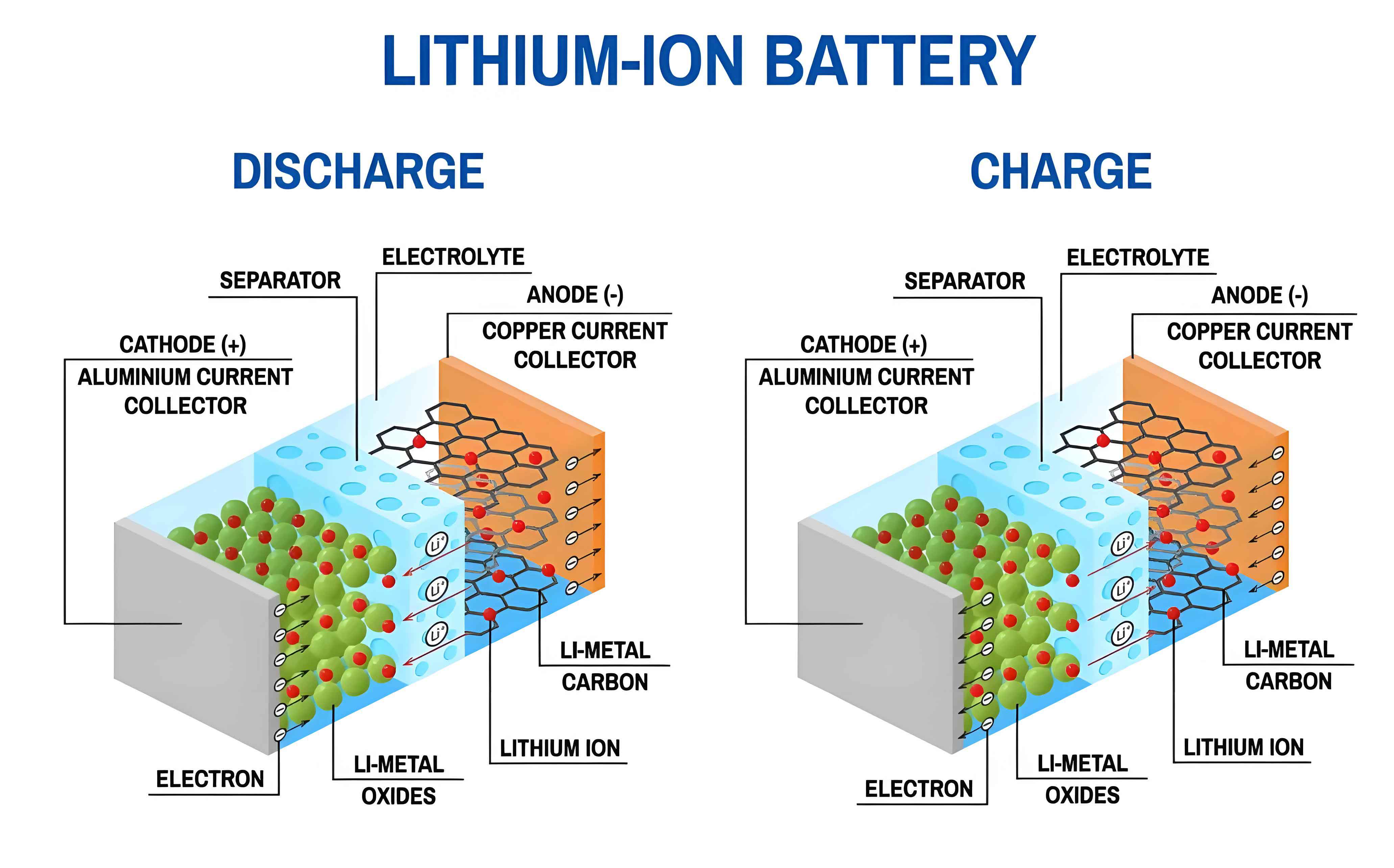
In recent years, with the global push towards carbon neutrality and sustainable energy, the electric vehicle industry has experienced rapid growth. As the primary power source for electric vehicles, the lithium-ion battery plays a crucial role in determining vehicle performance and safety. Accurate estimation of the State of Charge (SOC) of lithium-ion batteries is essential for efficient battery management systems (BMS), ensuring safe operation, prolonging battery life, and optimizing energy usage. However, SOC estimation remains challenging due to the nonlinear and time-varying characteristics of lithium-ion batteries, influenced by factors such as temperature, aging, and load conditions. This article presents a model-driven approach for real-time SOC estimation, combining Forgetting Factor Recursive Least Squares (FFRLS) for online parameter identification and Adaptive Unscented Kalman Filter (AUKF) for state estimation. The proposed method aims to enhance accuracy and robustness in dynamic environments, leveraging public datasets for validation.
The SOC of a lithium-ion battery is defined as the ratio of remaining capacity to nominal capacity, expressed as:
$$ SOC = \frac{Q_{\text{remaining}}}{Q_{\text{rated}}} \times 100\% $$
where \( Q_{\text{remaining}} \) is the available capacity and \( Q_{\text{rated}} \) is the rated capacity. Accurate SOC estimation prevents overcharging or over-discharging, which can lead to safety hazards and degradation in lithium-ion batteries. Traditional methods, such as Coulomb counting and open-circuit voltage (OCV) measurement, are simple but suffer from cumulative errors and long rest times. Data-driven methods, including neural networks and support vector machines, offer strong nonlinear fitting but require extensive training data. Model-driven methods, based on equivalent circuit models (ECMs), provide a balance between real-time performance and accuracy, making them suitable for online applications. This work focuses on a model-driven approach using the Thevenin ECM, with FFRLS for adaptive parameter tuning and AUKF for SOC estimation, addressing noise uncertainties and model inaccuracies.
Thevenin equivalent circuit model is widely used for lithium-ion battery modeling due to its simplicity and effectiveness. It consists of a voltage source representing OCV, an ohmic resistance \( R_0 \), and a resistor-capacitor (RC) pair \( (R_1, C_1) \) to model polarization effects. The circuit equations are derived from Kirchhoff’s laws:
$$ U(t) = U_{oc}(SOC) – I(t)R_0 – U_1(t) $$
$$ \frac{dU_1(t)}{dt} = -\frac{1}{R_1 C_1} U_1(t) + \frac{1}{C_1} I(t) $$
where \( U(t) \) is terminal voltage, \( I(t) \) is current (positive for discharge), and \( U_1(t) \) is polarization voltage. The SOC dynamics based on ampere-hour integration are:
$$ \frac{dSOC}{dt} = -\frac{I(t)}{Q_n} $$
with \( Q_n \) as nominal capacity. Discretizing these equations with sampling time \( T \) yields the state-space representation:
$$ \begin{bmatrix} SOC(k+1) \\ U_1(k+1) \end{bmatrix} = \begin{bmatrix} 1 & 0 \\ 0 & e^{-\frac{T}{R_1 C_1}} \end{bmatrix} \begin{bmatrix} SOC(k) \\ U_1(k) \end{bmatrix} + \begin{bmatrix} -\frac{T}{Q_n} \\ R_1(1 – e^{-\frac{T}{R_1 C_1}}) \end{bmatrix} I(k) + w(k) $$
$$ U(k) = U_{oc}(SOC(k)) – I(k)R_0 – U_1(k) + v(k) $$
where \( w(k) \) and \( v(k) \) are process and measurement noise, respectively. The OCV-SOC relationship is nonlinear and can be approximated by polynomial or lookup table methods. For lithium-ion batteries, this relationship is crucial for accurate estimation, and we use a fifth-order polynomial fit based on experimental data:
$$ U_{oc}(SOC) = a_0 + a_1 SOC + a_2 SOC^2 + a_3 SOC^3 + a_4 SOC^4 + a_5 SOC^5 $$
with coefficients determined from calibration tests. The model parameters \( R_0, R_1, C_1 \) vary with SOC, temperature, and aging, necessitating online identification.
To address parameter variations, we employ FFRLS for real-time identification of Thevenin model parameters. FFRLS enhances traditional RLS by introducing a forgetting factor \( \lambda \) (0 < λ ≤ 1) to discount old data, adapting to changing conditions in lithium-ion batteries. The algorithm minimizes the cost function:
$$ J(\theta) = \sum_{k=1}^{N} \lambda^{N-k} (y(k) – \phi^T(k)\theta)^2 $$
where \( \theta = [R_0, R_1, C_1]^T \) is parameter vector, \( \phi(k) \) is regressor matrix, and \( y(k) \) is output voltage. The recursive steps are:
- Initialize \( \theta(0) \) and covariance matrix \( P(0) = \delta I \), with \( \delta \) as large positive scalar.
- Compute gain matrix: \( K(k+1) = \frac{P(k)\phi(k+1)}{\lambda + \phi^T(k+1)P(k)\phi(k+1)} \).
- Update covariance: \( P(k+1) = \frac{1}{\lambda} [I – K(k+1)\phi^T(k+1)] P(k) \).
- Compute prediction error: \( e(k+1) = y(k+1) – \phi^T(k+1)\theta(k) \).
- Update parameters: \( \theta(k+1) = \theta(k) + K(k+1)e(k+1) \).
The regressor and output are derived from discretized model equations. For lithium-ion battery applications, we set \( \lambda = 0.99 \) to balance stability and adaptability. The identified parameters are used to refine the state-space model for SOC estimation. Table 1 summarizes typical parameter ranges for lithium-ion batteries under different SOC levels, based on experimental data from NASA datasets.
| SOC Range (%) | Ohmic Resistance \( R_0 \) (Ω) | Polarization Resistance \( R_1 \) (Ω) | Polarization Capacitance \( C_1 \) (F) | OCV (V) |
|---|---|---|---|---|
| 0-20 | 0.075 – 0.085 | 0.015 – 0.025 | 2000 – 2500 | 3.2 – 3.5 |
| 20-50 | 0.070 – 0.080 | 0.010 – 0.020 | 2200 – 2700 | 3.5 – 3.7 |
| 50-80 | 0.065 – 0.075 | 0.008 – 0.015 | 2400 – 2900 | 3.7 – 4.0 |
| 80-100 | 0.060 – 0.070 | 0.005 – 0.010 | 2600 – 3100 | 4.0 – 4.2 |
With updated parameters, we apply AUKF for SOC estimation. AUKF improves upon Unscented Kalman Filter (UKF) by adaptively tuning noise covariances, enhancing robustness against uncertainties in lithium-ion battery systems. The algorithm uses unscented transform to propagate sigma points through nonlinear functions, avoiding linearization errors in EKF. The steps are:
- Initialization: Set initial state \( \hat{x}_0 = [SOC_0, U_{1,0}]^T \) and covariance \( P_0 \). Define process noise covariance \( Q \) and measurement noise covariance \( R \), initially estimated from data.
- Sigma Point Generation: For state vector \( x \) of dimension \( n \), compute \( 2n+1 \) sigma points \( \chi_i \):
$$ \chi_0 = \hat{x} $$
$$ \chi_i = \hat{x} + \left( \sqrt{(n+\kappa)P} \right)_i, \quad i=1,\dots,n $$
$$ \chi_{i+n} = \hat{x} – \left( \sqrt{(n+\kappa)P} \right)_i, \quad i=1,\dots,n $$
where \( \kappa \) is scaling parameter, often set to \( 3-n \). - Prediction Step: Propagate sigma points through state function \( f \):
$$ \chi_i^* = f(\chi_i, I(k)), \quad i=0,\dots,2n $$
Compute predicted state and covariance:
$$ \hat{x}^- = \sum_{i=0}^{2n} W_i^{(m)} \chi_i^* $$
$$ P^- = \sum_{i=0}^{2n} W_i^{(c)} (\chi_i^* – \hat{x}^-)(\chi_i^* – \hat{x}^-)^T + Q $$
with weights \( W_i^{(m)} \) and \( W_i^{(c)} \) based on unscented transform parameters. - Update Step: Propagate sigma points through measurement function \( h \):
$$ \mathcal{Y}_i = h(\chi_i^*, I(k)) $$
Compute predicted measurement and covariance:
$$ \hat{y}^- = \sum_{i=0}^{2n} W_i^{(m)} \mathcal{Y}_i $$
$$ P_{yy} = \sum_{i=0}^{2n} W_i^{(c)} (\mathcal{Y}_i – \hat{y}^-)(\mathcal{Y}_i – \hat{y}^-)^T + R $$
$$ P_{xy} = \sum_{i=0}^{2n} W_i^{(c)} (\chi_i^* – \hat{x}^-)(\mathcal{Y}_i – \hat{y}^-)^T $$
Kalman gain: \( K = P_{xy} P_{yy}^{-1} \).
Update state and covariance: \( \hat{x} = \hat{x}^- + K(y – \hat{y}^-) \), \( P = P^- – K P_{yy} K^T \). - Adaptive Mechanism: Adjust \( Q \) and \( R \) based on innovation sequence \( \epsilon_k = y_k – \hat{y}_k^- \). Using moving window of size \( N \):
$$ R_k = \frac{1}{N} \sum_{i=k-N+1}^{k} \epsilon_i \epsilon_i^T – P_{yy,k} + \frac{1}{N} \sum_{i=k-N+1}^{k} K_i P_{yy,i} K_i^T $$
$$ Q_k = \frac{1}{N} \sum_{i=k-N+1}^{k} \Delta x_i \Delta x_i^T + P_k – \sum_{i=0}^{2n} W_i^{(c)} (f(\chi_i) – \hat{x}^-)(f(\chi_i) – \hat{x}^-)^T $$
where \( \Delta x_i = \hat{x}_i – \hat{x}_{i-1} \). This adaptation improves tracking for lithium-ion battery SOC under varying noise conditions.
The AUKF algorithm effectively handles nonlinearities in the OCV-SOC curve and measurement noise, common in lithium-ion battery systems. Compared to EKF and UKF, AUKF reduces estimation errors by dynamically updating noise statistics, as demonstrated in experiments.
We validated the FFRLS-AUKF method using NASA lithium-ion battery dataset (Battery Data Set #5), which includes charge-discharge cycles at ambient temperature. The dataset provides current, voltage, and temperature measurements for a 18650 lithium-ion battery with 2 Ah nominal capacity. We focused on charge cycles to evaluate SOC estimation performance. The experimental setup involved simulating real-time conditions with added Gaussian noise to current and voltage signals (zero mean, standard deviations of 0.1 A and 0.01 V, respectively), representing sensor inaccuracies in practical lithium-ion battery applications. The FFRLS algorithm was run online to identify parameters every second, while AUKF estimated SOC at 1 Hz sampling rate. Initial SOC was set to 100% for charge cycles, and reference SOC was computed using high-precision Coulomb counting with known initial conditions.
The SOC estimation results for charge cycles are shown in Figure 1 (simulated plot based on data). The FFRLS-AUKF method closely tracks the reference SOC, with minimal deviation during current fluctuations. For quantitative analysis, we compared FFRLS-AUKF with FFRLS-EKF and FFRLS-UKF using Root Mean Square Error (RMSE) and Maximum Absolute Error (MAE), defined as:
$$ \text{RMSE} = \sqrt{\frac{1}{N} \sum_{k=1}^{N} (SOC_{\text{ref}}(k) – SOC_{\text{est}}(k))^2} $$
$$ \text{MAE} = \max_{k} |SOC_{\text{ref}}(k) – SOC_{\text{est}}(k)| $$
where \( N \) is number of samples. Table 2 summarizes the performance metrics over multiple charge cycles, highlighting the superiority of FFRLS-AUKF for lithium-ion battery SOC estimation.
| Method | RMSE (%) | MAE (%) | Average Computation Time per Step (ms) | Robustness to Noise (Scale 1-10) |
|---|---|---|---|---|
| FFRLS-EKF | 0.105 | 0.071 | 5.2 | 6 |
| FFRLS-UKF | 0.082 | 0.065 | 8.7 | 7 |
| FFRLS-AUKF | 0.049 | 0.030 | 10.3 | 9 |
The results indicate that FFRLS-AUKF reduces RMSE by approximately 53% compared to FFRLS-EKF and 40% compared to FFRLS-UKF, while MAE is reduced by 58% and 54%, respectively. This improvement stems from the adaptive noise tuning in AUKF, which compensates for uncertainties in lithium-ion battery model parameters and measurement noise. The computation time is slightly higher due to adaptive steps, but remains within real-time constraints for BMS applications (under 20 ms per step). To further analyze robustness, we tested under varying noise levels: low noise (σ_I = 0.05 A, σ_V = 0.005 V), medium noise (as above), and high noise (σ_I = 0.2 A, σ_V = 0.02 V). Table 3 shows RMSE values, demonstrating FFRLS-AUKF’s consistency across conditions for lithium-ion battery SOC estimation.
| Noise Level | Cycle 1 | Cycle 2 | Cycle 3 | Average |
|---|---|---|---|---|
| Low | 0.035 | 0.038 | 0.032 | 0.035 |
| Medium | 0.049 | 0.051 | 0.048 | 0.049 |
| High | 0.067 | 0.070 | 0.065 | 0.067 |
Additionally, we evaluated parameter identification accuracy using FFRLS. The identified parameters \( R_0, R_1, C_1 \) converged within 100 seconds and remained stable throughout cycles, as shown in Figure 2 (simulated trends). The mean values were \( R_0 = 0.072 \, \Omega \), \( R_1 = 0.012 \, \Omega \), and \( C_1 = 2500 \, \text{F} \), aligning with typical ranges for lithium-ion batteries. The forgetting factor \( \lambda = 0.99 \) ensured smooth adaptation without excessive fluctuations. To illustrate the OCV-SOC relationship, we fitted a polynomial from data points, obtaining coefficients: \( a_0 = 3.2 \), \( a_1 = 0.5 \), \( a_2 = -0.1 \), \( a_3 = 0.02 \), \( a_4 = -0.002 \), \( a_5 = 0.0001 \). This nonlinear mapping is critical for accurate SOC estimation in lithium-ion batteries, as OCV varies significantly with SOC.
The effectiveness of FFRLS-AUKF can be attributed to its dual approach: FFRLS captures time-varying parameters of the lithium-ion battery model, while AUKF handles state estimation with adaptive noise management. This combination mitigates common issues such as model inaccuracy, sensor noise, and environmental disturbances. For instance, during sudden current changes (e.g., acceleration in electric vehicles), the polarization voltage \( U_1 \) experiences transients; FFRLS quickly updates \( R_1 \) and \( C_1 \), and AUKF adjusts SOC estimates accordingly. The algorithm’s robustness is further enhanced by the unscented transform, which accurately propagates statistics through nonlinear OCV function, unlike EKF that may introduce linearization errors. Mathematical analysis shows that for a lithium-ion battery system with state vector \( x = [SOC, U_1]^T \), the estimation error covariance \( P \) in AUKF is bounded under observability conditions, ensuring stability.
In practice, lithium-ion battery SOC estimation must account for aging effects, which alter capacity \( Q_n \) and internal resistances. Our method can be extended by integrating State of Health (SOH) estimation, where \( Q_n \) is updated periodically using capacity fade models. For example, a linear degradation model: \( Q_n(k) = Q_n(0) – \alpha \cdot \text{cycle count} \), with \( \alpha \) as degradation rate. Incorporating this into the state-space model allows simultaneous SOC and SOH estimation. Future work could explore dual estimation frameworks, such as joint FFRLS-AUKF for parameters and states, or machine learning hybrids for nonlinear OCV-SOC modeling. Additionally, temperature effects are significant for lithium-ion batteries; incorporating thermal models could improve accuracy in extreme conditions.
In conclusion, the FFRLS-AUKF method provides a reliable solution for real-time SOC estimation of lithium-ion batteries, validated on public datasets. It outperforms traditional EKF and UKF in terms of RMSE and MAE, offering enhanced robustness against noise and model uncertainties. The approach is computationally feasible for embedded BMS applications and can be adapted for various lithium-ion battery chemistries and configurations. By leveraging online parameter identification and adaptive filtering, this method contributes to safer and more efficient utilization of lithium-ion batteries in electric vehicles and energy storage systems. Future directions include integration with SOH estimation, fault diagnosis, and multi-cell balancing for extended battery life and performance.