
In the realm of modern energy storage systems, lithium-ion batteries have emerged as a cornerstone due to their high energy density and power output capabilities. As we delve into the intricacies of battery management, it becomes evident that the gradual degradation of capacity and power over time poses significant challenges for reliability and safety. The assessment of State of Health (SOH) and prediction of Remaining Useful Life (RUL) are thus critical for optimizing the lifecycle management of lithium-ion batteries, spanning from design and manufacturing to deployment and second-life applications. Traditional machine learning approaches have been applied to simulate battery performance and estimate states, but they often fall short in quantifying prediction uncertainty. Given the complex, multi-physics nature of lithium-ion battery degradation—involving coupled factors like solid electrolyte interphase (SEI) growth, electrode cracking, and lithium plating—there is a pressing need for robust probabilistic frameworks that can handle data variability and provide reliable confidence intervals. In this article, we explore the integration of probabilistic machine learning for lithium-ion battery health diagnosis and prognosis, emphasizing uncertainty quantification, algorithmic selection, and practical implementation steps. We will use tables and formulas to summarize key concepts, ensuring a comprehensive overview that addresses the limitations of deterministic models while highlighting future directions for intelligent energy storage management.
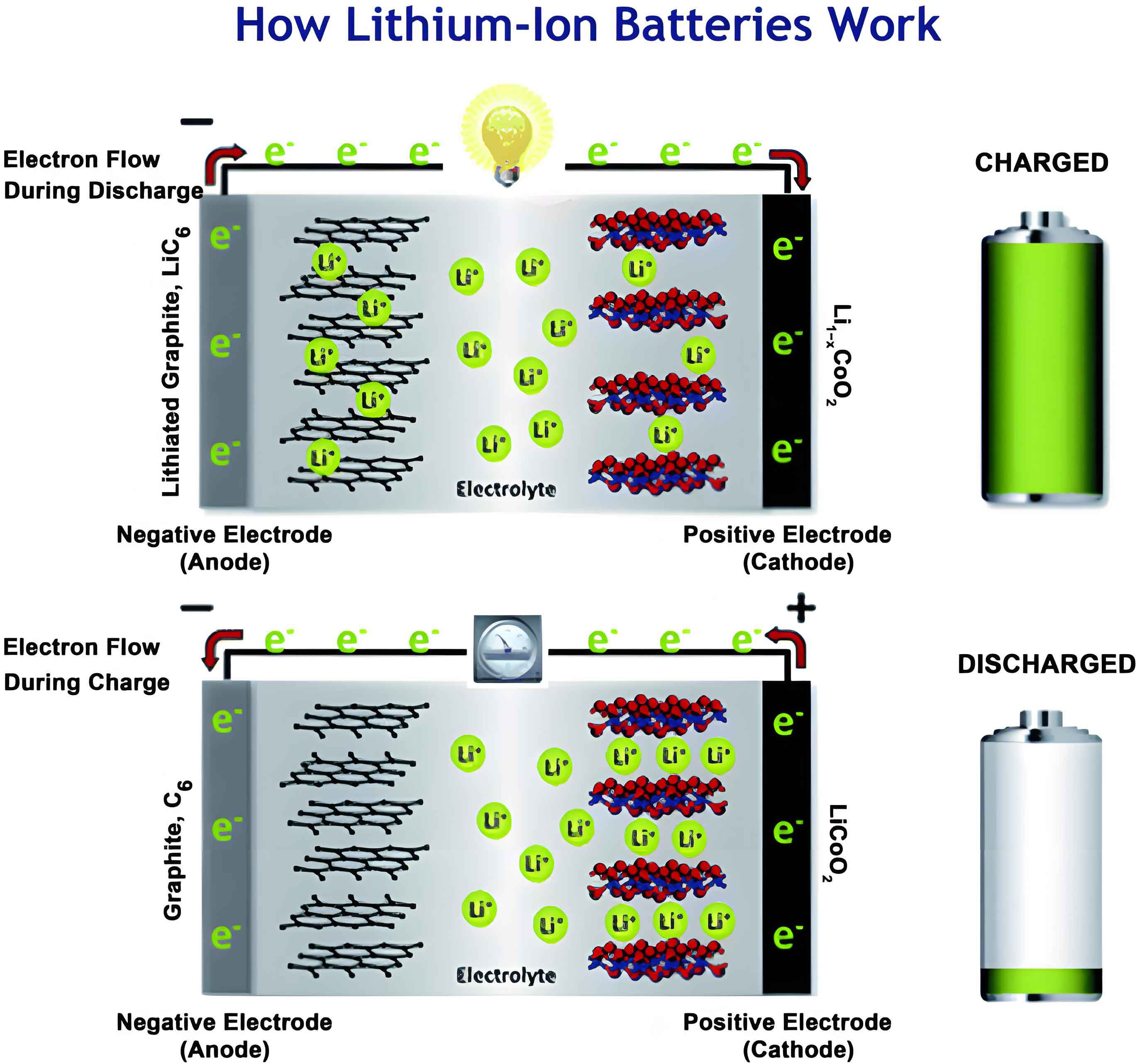
The widespread adoption of lithium-ion batteries in grid-scale storage and electric vehicles has intensified research into their aging mechanisms. A lithium-ion battery’s health is primarily gauged by its SOH, defined as the ratio of current maximum capacity to initial capacity, often expressed as: $$ \text{SOH} = \frac{C_{\text{current}}}{C_{\text{initial}}} \times 100\% $$ where $C_{\text{current}}$ is the present available capacity and $C_{\text{initial}}$ is the nominal capacity. However, this metric alone does not capture the underlying degradation processes, which are stochastic and influenced by operational conditions such as temperature, charge-discharge rates, and depth of discharge (DOD). For instance, SEI film growth on the anode surface follows a parabolic growth law, which can be modeled as: $$ Q_{\text{SEI}}(t) = k \cdot \sqrt{t} $$ where $Q_{\text{SEI}}$ is the charge consumed by SEI formation, $k$ is a rate constant dependent on temperature and voltage, and $t$ is time. This reaction irreversibly consumes active lithium ions, leading to capacity fade. Coupled with mechanical stress from electrode volume changes during cycling, it creates a nonlinear degradation trajectory that complicates prediction. We argue that probabilistic machine learning offers a paradigm shift by not only predicting point estimates but also quantifying uncertainties, thereby enhancing decision-making in battery health management for lithium-ion batteries.
To understand the degradation mechanisms in lithium-ion batteries, we must consider multi-scale phenomena. The table below summarizes key degradation modes and their impacts on SOH and RUL for lithium-ion batteries:
| Degradation Mode | Primary Cause | Effect on Capacity | Uncertainty Factors |
|---|---|---|---|
| SEI Growth | Electrolyte decomposition at anode | Linear to parabolic fade | Temperature, SOC, cycle number |
| Lithium Plating | Low-temperature or high-rate charging | Sudden capacity drop | Charge rate, temperature gradients |
| Electrode Cracking | Mechanical stress from cycling | Increased impedance and fade | DOD, cycle frequency, material properties |
| Active Material Loss | Structural disintegration of electrodes | Gradual capacity decline | Operating voltage limits, aging history |
These mechanisms interact in complex ways, making deterministic models inadequate. For example, the combined effect of SEI growth and lithium plating can be described by a coupled differential equation: $$ \frac{dC}{dt} = -\alpha \cdot \exp\left(-\frac{E_a}{RT}\right) \cdot C^{\beta} – \gamma \cdot I_{\text{charge}} \cdot H(T_{\text{low}}) $$ where $C$ is capacity, $\alpha, \beta, \gamma$ are constants, $E_a$ is activation energy, $R$ is the gas constant, $T$ is temperature, $I_{\text{charge}}$ is charging current, and $H$ is a Heaviside function for low-temperature conditions. The stochastic nature of these parameters necessitates probabilistic approaches to capture variability across different lithium-ion battery cells and operating conditions.
In health diagnosis and prediction for lithium-ion batteries, we categorize the core problems into two modules: real-time state diagnosis and lifetime prognosis. The real-time module focuses on estimating current SOH and identifying degradation mechanisms, while the prognosis module aims to predict future SOH trajectories and RUL. Below, we outline these modules with probabilistic machine learning techniques.
Real-Time State Diagnosis Module: This involves continuous monitoring of voltage, current, and temperature data from battery management systems (BMS). Key tasks include SOH estimation and multi-mode degradation diagnosis. For SOH estimation, we can use Bayesian linear regression to infer capacity from partial charge curves. The model assumes: $$ y = \mathbf{w}^T \mathbf{x} + \epsilon $$ where $y$ is the capacity estimate, $\mathbf{x}$ is a feature vector (e.g., constant-voltage phase duration, differential voltage peaks), $\mathbf{w}$ is a weight vector with a prior distribution $p(\mathbf{w})$, and $\epsilon \sim \mathcal{N}(0, \sigma^2)$ is Gaussian noise. By applying Bayes’ theorem: $$ p(\mathbf{w} | \mathbf{X}, \mathbf{y}) = \frac{p(\mathbf{y} | \mathbf{X}, \mathbf{w}) p(\mathbf{w})}{p(\mathbf{y} | \mathbf{X})} $$ we obtain a posterior distribution over weights, yielding predictive distributions with confidence intervals. For multi-mode diagnosis, we employ multi-task Gaussian processes to jointly estimate contributions from SEI growth, lithium inventory loss, and active material loss. The covariance function can be defined as: $$ k(\mathbf{x}_i, \mathbf{x}_j) = \sigma_f^2 \exp\left(-\frac{|\mathbf{x}_i – \mathbf{x}_j|^2}{2l^2}\right) + \sigma_n^2 \delta_{ij} $$ where $\sigma_f^2$ is signal variance, $l$ is length-scale, $\sigma_n^2$ is noise variance, and $\delta_{ij}$ is the Kronecker delta. This allows uncertainty quantification for each degradation mode, crucial for targeted maintenance of lithium-ion batteries.
Lifetime Prognosis Module: This module addresses RUL prediction, SOH trajectory forecasting, and early-life prediction. For RUL prediction, we use deep temporal models like Temporal Convolutional Networks (TCN) combined with Gaussian Processes (GP). The TCN extracts features from sliding windows of capacity fade sequences, and the GP models the residual uncertainty. The RUL is defined as: $$ \text{RUL} = t_{\text{end}} – t_{\text{current}} $$ where $t_{\text{end}}$ is the predicted cycle number when SOH falls below a threshold (e.g., 80%). The predictive distribution for capacity at cycle $t$ is given by: $$ p(C_t | \mathbf{X}_{\leq t}) = \int p(C_t | f_t) p(f_t | \mathbf{X}_{\leq t}) df_t $$ where $f_t$ is the latent function from the GP. For trajectory prediction, we employ sequence-to-sequence models with Monte Carlo dropout to generate probabilistic forecasts. Early-life prediction leverages transfer learning: we extract features from initial cycles (e.g., Coulombic efficiency, incremental capacity curve shapes) and use Bayesian neural networks to predict full degradation curves. The loss function often includes a Kullback-Leibler divergence term to regularize uncertainty: $$ \mathcal{L} = \mathbb{E}_{q(\theta)}[\log p(\mathbf{y} | \mathbf{X}, \theta)] – \text{KL}(q(\theta) || p(\theta)) $$ where $\theta$ are model parameters, $q(\theta)$ is the variational posterior, and $p(\theta)$ is the prior. This framework enhances generalization across diverse lithium-ion battery datasets.
To compare different probabilistic algorithms for lithium-ion battery health management, we present the following table based on key metrics:
| Algorithm | Prediction Accuracy (RMSE) | Uncertainty Calibration (ECE) | Computational Efficiency | Data Size Suitability | Noise Robustness |
|---|---|---|---|---|---|
| Gaussian Process Regression (GPR) | 0.02–0.05 | 0.01–0.03 | O(n³) for training | Small to medium (N < 10⁴) | High |
| Bayesian Neural Network (BNN) | 0.01–0.03 | 0.02–0.05 | O(n) for inference | Medium to large (N ≥ 10³) | Medium |
| Relevance Vector Machine (RVM) | 0.03–0.06 | 0.01–0.04 | O(n²) for training | Small (N < 10³) | High |
| Deep Ensemble Learning | 0.01–0.02 | 0.01–0.02 | O(m·n) for m models | Large (N ≥ 10⁴) | Very High |
| Bootstrap Aggregating | 0.02–0.04 | 0.03–0.06 | O(b·n) for b bootstraps | Medium (N ~ 10³–10⁴) | Medium |
Note: RMSE (Root Mean Square Error) in normalized capacity units, ECE (Expected Calibration Error) in probability units. Data from empirical studies on lithium-ion battery aging datasets. The choice of algorithm depends on application constraints; for instance, GPR is ideal for small datasets with high uncertainty quantification needs, while BNNs scale better for large-scale monitoring of lithium-ion batteries.
Despite the advantages of deep learning in automated feature extraction, it suffers from overfitting on small samples and black-box limitations. In contrast, probabilistic deep learning incorporates uncertainty through methods like Bayesian inference or dropout variational inference. For a lithium-ion battery, the predictive distribution from a Bayesian neural network can be approximated using Monte Carlo dropout: $$ p(y^* | \mathbf{x}^*, \mathbf{X}, \mathbf{y}) \approx \frac{1}{T} \sum_{t=1}^T p(y^* | \mathbf{x}^*, \hat{\theta}_t) $$ where $\hat{\theta}_t$ are sampled parameters from dropout during $T$ forward passes. This yields both mean predictions and variance, which can be decomposed into aleatoric (data) and epistemic (model) uncertainty: $$ \text{Var}(y^*) = \underbrace{\frac{1}{T} \sum_{t=1}^T \hat{\sigma}_t^2}_{\text{aleatoric}} + \underbrace{\frac{1}{T} \sum_{t=1}^T (\hat{\mu}_t – \bar{\mu})^2}_{\text{epistemic}} $$ where $\hat{\mu}_t$ and $\hat{\sigma}_t^2$ are mean and variance from each dropout sample, and $\bar{\mu}$ is the ensemble mean. Such decomposition is vital for identifying when predictions are unreliable, especially in safety-critical applications involving lithium-ion batteries.
The application of probabilistic machine learning to lithium-ion battery health diagnosis and prediction follows a systematic workflow. We detail the steps below, incorporating formulas and best practices.
Step 1: Input-Output Variable Definition. Define feature vectors $\mathbf{x}$ from BMS data, such as voltage curves during constant-current charging, temperature profiles, and impedance measurements. For example, we can extract features like time to reach 80% SOC ($t_{80}$) or curvature of voltage relaxation. The output $y$ is typically SOH or RUL. A common model is: $$ y = f(\mathbf{x}) + \epsilon, \quad \epsilon \sim \mathcal{N}(0, \sigma^2) $$ where $f$ is a probabilistic function to be learned.
Step 2: Dataset Construction and Partitioning. Collect data from multiple lithium-ion battery cells under varied conditions. Use cell-level splitting to prevent data leakage: 70% of cells for training, 15% for validation, and 15% for testing. Include out-of-distribution samples (e.g., different temperatures or new battery chemistries) to assess generalization. The dataset size $N$ should be large enough to support uncertainty estimation; for lithium-ion batteries, we recommend $N \geq 1000$ cycles for robust probabilistic modeling.
Step 3: Algorithm Selection and Training. Choose algorithms based on criteria from the earlier table. For instance, if data is limited ($N < 300$), use GPR with a Matérn kernel: $$ k_{\text{Matérn}}(r) = \frac{2^{1-\nu}}{\Gamma(\nu)} \left( \frac{\sqrt{2\nu} r}{l} \right)^\nu K_\nu \left( \frac{\sqrt{2\nu} r}{l} \right) $$ where $r = |\mathbf{x}_i – \mathbf{x}_j|$, $\nu$ controls smoothness, and $K_\nu$ is a modified Bessel function. Train using maximum marginal likelihood or variational inference. For larger datasets, employ BNNs with stochastic gradient Markov chain Monte Carlo (SG-MCMC) for sampling posterior weights.
Step 4: Model Validation and Uncertainty Calibration. Evaluate on test sets using metrics like Mean Absolute Percentage Error (MAPE) for accuracy: $$ \text{MAPE} = \frac{100\%}{n} \sum_{i=1}^n \left| \frac{y_i – \hat{y}_i}{y_i} \right| $$ and interval coverage probability (ICP) for uncertainty: $$ \text{ICP} = \frac{1}{n} \sum_{i=1}^n \mathbb{I}(y_i \in [\hat{y}_i – z_{\alpha/2} \hat{\sigma}_i, \hat{y}_i + z_{\alpha/2} \hat{\sigma}_i]) $$ where $\mathbb{I}$ is an indicator function, $z_{\alpha/2}$ is the critical value for a $(1-\alpha)$ confidence interval (e.g., 1.96 for 95%), and $\hat{\sigma}_i$ is predicted standard deviation. For lithium-ion battery SOH prediction, we target MAPE < 5% and ICP ≥ 90%.
Step 5: Deployment and Continuous Learning. Deploy the model in BMS for real-time monitoring. Incorporate online Bayesian updating to adapt to new data: $$ p(\theta | \mathbf{y}_{\text{new}}) \propto p(\mathbf{y}_{\text{new}} | \theta) p(\theta | \mathbf{y}_{\text{old}}) $$ This ensures the model evolves with battery aging, crucial for long-term reliability of lithium-ion batteries.
To illustrate the workflow, consider a case study on lithium-ion battery RUL prediction. We simulate capacity fade using an empirical model with noise: $$ C_n = C_0 \cdot \exp(-\alpha n^\beta) + \epsilon_n, \quad \epsilon_n \sim \mathcal{N}(0, \sigma_c^2) $$ where $n$ is cycle number, $\alpha$ and $\beta$ are degradation parameters. Using GPR, we predict future cycles and compute RUL distributions. The results can be summarized in a table:
| Cycle Number | True Capacity (Ah) | Predicted Mean (Ah) | 95% Confidence Interval (Ah) | RUL Estimate (cycles) |
|---|---|---|---|---|
| 100 | 4.85 | 4.83 | [4.78, 4.88] | 450 ± 50 |
| 200 | 4.70 | 4.68 | [4.62, 4.74] | 300 ± 40 |
| 300 | 4.50 | 4.52 | [4.45, 4.59] | 150 ± 30 |
Such probabilistic outputs enable risk-aware decisions, like scheduling maintenance before a lithium-ion battery reaches critical degradation.
Looking ahead, the future of lithium-ion battery health management lies in developing interpretable probabilistic models that integrate physical mechanisms. Physics-informed neural networks (PINNs) are promising, as they embed differential equations governing battery dynamics into loss functions. For example, we can combine Fick’s law of diffusion with a Bayesian framework: $$ \frac{\partial c}{\partial t} = D \nabla^2 c + R(c, \theta) $$ where $c$ is lithium concentration, $D$ is diffusion coefficient, and $R$ represents reaction terms. By learning parameters $\theta$ as distributions, we quantify uncertainties in physical processes. Additionally, hybrid models that fuse data-driven approaches with electrochemical models (e.g., Doyle-Fuller-Newman models) can enhance predictability for lithium-ion batteries under diverse operating conditions. We also envision federated learning for privacy-preserving collaboration across battery fleets, leveraging probabilistic aggregation to improve global models while respecting data locality.
In conclusion, probabilistic machine learning transforms lithium-ion battery health assessment and degradation prediction by quantifying uncertainties that deterministic methods overlook. Through algorithms like Gaussian processes, Bayesian neural networks, and deep ensembles, we can achieve robust SOH estimation and RUL forecasting with confidence intervals. The application steps—from data curation to algorithm selection and validation—provide a roadmap for implementation in real-world energy storage systems. As lithium-ion batteries continue to power our grid and transportation, advancing probabilistic frameworks will be key to ensuring their safety, longevity, and efficiency. We encourage further research into explainable AI and physics-integrated models to unlock the full potential of intelligent battery management for lithium-ion batteries.