
I investigate the behavior and control of solar inverters when the utility grid is subjected to asymmetric faults. In modern photovoltaic generation, solar inverters are the central interface between the direct-current photovoltaic source and the alternating-current grid. Their control determines whether the photovoltaic plant can remain connected, how much active and reactive power is delivered, how well the direct-current link voltage is regulated, and how clean the injected current remains. When the grid is balanced, conventional vector control in a positive-sequence synchronous reference frame is usually sufficient. When the grid becomes unbalanced, however, negative-sequence voltage and current components appear, and the behavior of solar inverters changes fundamentally. I therefore develop a predictive current control method for solar inverters under asymmetric grid faults, and I evaluate its ability to suppress active power ripple and negative-sequence current without decomposing the grid current into positive and negative sequences.
The central motivation is practical. For solar inverters, asymmetric faults produce second-order power oscillations, direct-current link voltage pulsations, unbalanced three-phase currents, increased harmonic distortion, and possible stress on the direct-current bus capacitor. These effects reduce the quality of the power supplied by solar inverters and may degrade the lifetime of key components. A control method that can act directly in the stationary reference frame, avoid current sequence separation, and still provide fast dynamic response is highly attractive for solar inverters. I formulate such a method using a model predictive current controller and examine two control targets: minimizing active power ripple and minimizing negative-sequence current.
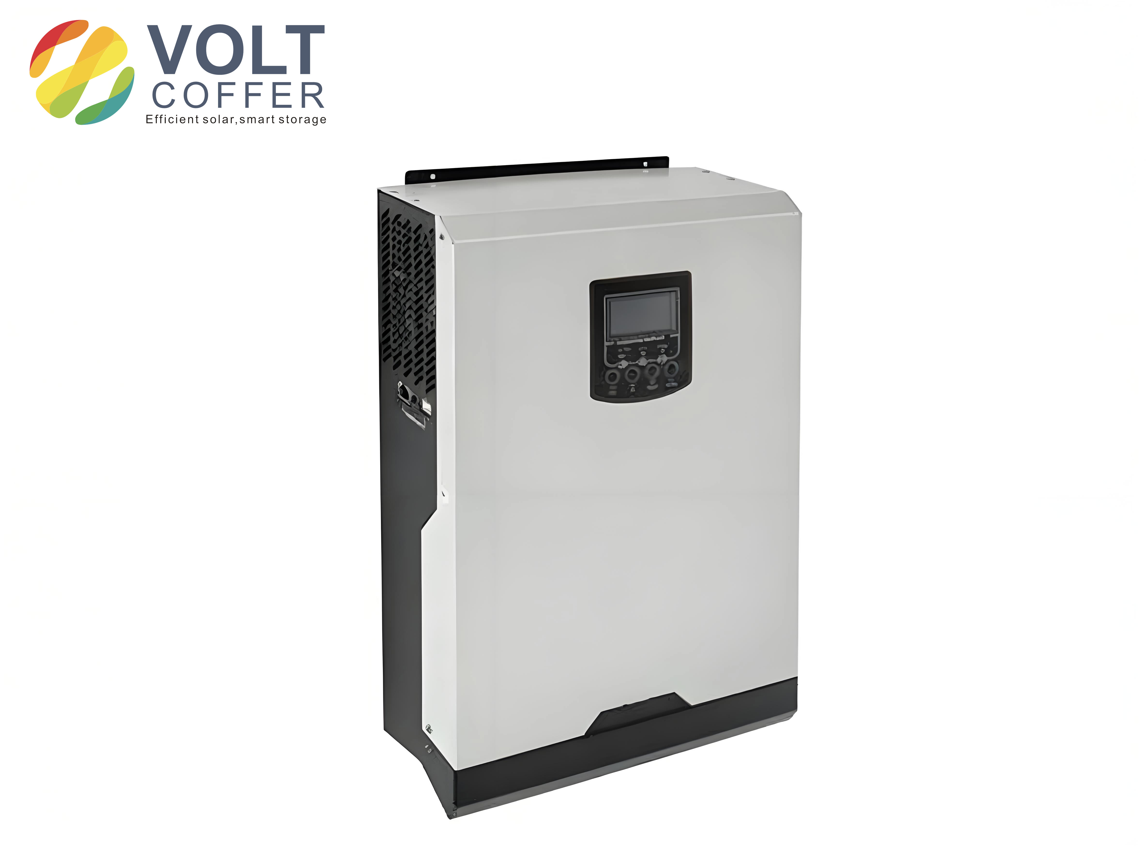
Dynamic Model of Solar Inverters Under Asymmetric Grid Conditions
I begin with the main circuit of a grid-connected photovoltaic system. The solar inverter is connected to the grid through a filter inductance and an equivalent series resistance. The direct-current side contains a capacitor and the photovoltaic array. The inverter output voltage is represented by \(U_{t,abc}\), the inverter output current by \(I_{abc}\), the grid voltage by \(U_{g,abc}\), and the direct-current voltage by \(U_{dc}\). Applying Kirchhoff voltage law in the three-phase stationary frame gives
$$U_{t,abc}=U_{g,abc}+L\frac{dI_{abc}}{dt}+R I_{abc}.$$
Transforming this equation into the two-phase stationary \(\alpha\beta\) frame yields
$$U_{t,\alpha\beta}=U_{g,\alpha\beta}+L\frac{dI_{\alpha\beta}}{dt}+R I_{\alpha\beta}.$$
When the grid voltage is asymmetric, every electrical quantity contains a positive-sequence component rotating counterclockwise at the synchronous angular speed \(\omega_0\) and a negative-sequence component rotating clockwise at the same speed. I express a general voltage or current vector \(F_{\alpha\beta}\) as
$$F_{\alpha\beta}=F^p_{\alpha\beta}+F^n_{\alpha\beta}=F^p_{dq}e^{j\theta}+F^n_{dq}e^{-j\theta},$$
where \(\theta=\omega_0 t\). The superscript \(p\) denotes the positive sequence, and the superscript \(n\) denotes the negative sequence. For the grid voltage, inverter voltage, and current, I write
$$U_{g,\alpha\beta}=U^p_{g,dq}e^{j\theta}+U^n_{g,dq}e^{-j\theta},$$
$$U_{t,\alpha\beta}=U^p_{t,dq}e^{j\theta}+U^n_{t,dq}e^{-j\theta},$$
$$I_{\alpha\beta}=I^p_{dq}e^{j\theta}+I^n_{dq}e^{-j\theta}.$$
Substituting these expressions into the \(\alpha\beta\) model separates the positive-sequence and negative-sequence dynamics. The positive-sequence equation in the counterclockwise synchronous frame becomes
$$U^p_{t,dq}=U^p_{g,dq}+L\frac{dI^p_{dq}}{dt}+j\omega_0 L I^p_{dq},$$
and the negative-sequence equation in the clockwise synchronous frame becomes
$$U^n_{t,dq}=U^n_{g,dq}+L\frac{dI^n_{dq}}{dt}-j\omega_0 L I^n_{dq}.$$
These equations show that negative-sequence components are not naturally controlled by a standard proportional-integral regulator operating only in the positive-sequence synchronous frame. If I use only positive-sequence control for solar inverters, the negative-sequence current is not directly regulated, and the active and reactive power delivered by the solar inverters contain oscillatory terms.
The complex power delivered to the grid is
$$S=\frac{3}{2}U_{g,\alpha\beta}I_{\alpha\beta}^*.$$
Expanding this expression with positive-sequence and negative-sequence components gives the active power \(P\) and reactive power \(Q\) as
$$P=P_0+P_{c2}\cos(2\omega_0 t)+P_{s2}\sin(2\omega_0 t),$$
$$Q=Q_0+Q_{c2}\cos(2\omega_0 t)+Q_{s2}\sin(2\omega_0 t).$$
The six power components can be arranged in matrix form as follows:
$$
\begin{bmatrix}
P_0\\
P_{c2}\\
P_{s2}\\
Q_0\\
Q_{c2}\\
Q_{s2}
\end{bmatrix}
=
\frac{3}{2}
\begin{bmatrix}
U^p_{gd} & U^p_{gq} & U^n_{gd} & U^n_{gq}\\
U^n_{gd} & U^n_{gq} & U^p_{gd} & U^p_{gq}\\
U^n_{gq} & -U^n_{gd} & -U^p_{gq} & U^p_{gd}\\
U^p_{gq} & -U^p_{gd} & U^n_{gq} & -U^n_{gd}\\
U^n_{gq} & -U^n_{gd} & U^p_{gq} & -U^p_{gd}\\
-U^n_{gd} & -U^n_{gq} & U^p_{gd} & U^p_{gq}
\end{bmatrix}
\begin{bmatrix}
I^p_d\\
I^p_q\\
I^n_d\\
I^n_q
\end{bmatrix}.
$$
This matrix is important for solar inverters because it reveals the coupling between sequence currents and power oscillations. The active power has a constant term and two second-order oscillatory terms. The reactive power also has a constant term and two second-order oscillatory terms. In an asymmetric grid, it is generally impossible to eliminate both active and reactive power oscillations simultaneously by controlling only the positive-sequence and negative-sequence currents. I therefore select a single control objective at a time, according to the priorities of the solar inverters and the grid operator.
| Power component | Meaning | Effect on solar inverters |
|---|---|---|
| \(P_0\) | Average active power | Determines photovoltaic energy delivery |
| \(P_{c2},P_{s2}\) | Second-order active power ripple | Produces direct-current link voltage pulsation |
| \(Q_0\) | Average reactive power | Supports voltage and reactive power requirements |
| \(Q_{c2},Q_{s2}\) | Second-order reactive power ripple | Affects power quality and converter stress |
| \(I^p_d,I^p_q\) | Positive-sequence current in synchronous frame | Controls average active and reactive power |
| \(I^n_d,I^n_q\) | Negative-sequence current in synchronous frame | Creates unbalanced grid current if uncontrolled |
Control Objectives for Solar Inverters
I consider two practical control objectives for solar inverters during asymmetric grid faults. The first objective is to suppress active power ripple. The second objective is to suppress negative-sequence current. The first objective protects the direct-current link and the photovoltaic source from second-order power pulsation. The second objective minimizes current unbalance and improves the quality of the current injected by the solar inverters.
If I choose to suppress active power ripple, I set the active power oscillation terms to zero:
$$P_{c2}=0, \qquad P_{s2}=0.$$
With the grid voltage oriented along the positive-sequence \(d\)-axis, I take
$$U^p_{gq}=0.$$
The reference values for the sequence currents are then
$$I^p_{d,ref}=\frac{P_{ref}}{1.5U^p_{gd}\left(1-k_{dd}^2-k_{qd}^2\right)},$$
$$I^p_{q,ref}=-\frac{Q_{ref}}{1.5U^p_{gd}\left(1-k_{dd}^2-k_{qd}^2\right)},$$
$$I^n_{d,ref}=-k_{dd}I^p_d-k_{qd}I^p_q,$$
$$I^n_{q,ref}=k_{dd}I^p_q-k_{qd}I^p_d,$$
where
$$k_{dd}=\frac{U^n_{gd}}{U^p_{gd}}, \qquad k_{qd}=\frac{U^n_{gq}}{U^p_{gd}}.$$
If I choose to suppress negative-sequence current, I set
$$I^n_{d,ref}=0, \qquad I^n_{q,ref}=0.$$
The positive-sequence current references are then
$$I^p_{d,ref}=\frac{P_{ref}}{1.5U^p_{gd}},$$
$$I^p_{q,ref}=-\frac{Q_{ref}}{1.5U^p_{gd}}.$$
For photovoltaic generation, the active power reference is usually obtained from a maximum power point tracking controller. I represent this by
$$P_{ref}=K_p\left(U_{MPPT}-U_{dc}\right)+K_i\int\left(U_{MPPT}-U_{dc}\right)dt.$$
I usually set the reactive power reference to zero when unity power factor operation is desired, but during grid support conditions the reactive current reference may be nonzero. The following table summarizes the two objectives and their reference conditions.
| Objective | Condition | Positive-sequence references | Negative-sequence references |
|---|---|---|---|
| Suppress active power ripple | \(P_{c2}=0, P_{s2}=0\) | Functions of \(P_{ref}\), \(Q_{ref}\), and voltage unbalance | \(I^n_{d,ref}=-k_{dd}I^p_d-k_{qd}I^p_q\), \(I^n_{q,ref}=k_{dd}I^p_q-k_{qd}I^p_d\) |
| Suppress negative-sequence current | \(I^n_{d,ref}=0, I^n_{q,ref}=0\) | \(I^p_{d,ref}=P_{ref}/(1.5U^p_{gd})\), \(I^p_{q,ref}=-Q_{ref}/(1.5U^p_{gd})\) | Zero |
Model Predictive Current Control for Solar Inverters
I use a model predictive current controller for the solar inverters. The controller predicts the future current for each possible switching state of the inverter and selects the switching state that minimizes a cost function. This approach is natural for solar inverters because the inverter has a finite number of switching states, and the prediction model can be written directly in the stationary \(\alpha\beta\) frame. It also avoids the need to separate the grid current into positive and negative sequences, because the current reference in the stationary frame already contains both sequences.
For a two-level three-phase inverter, I define the switching function \(g_i\), where \(i=a,b,c\), as
$$g_i=
\begin{cases}
1 & \text{upper switch on},\\
0 & \text{lower switch on}.
\end{cases}
$$
The inverter output voltage vector is
$$u_t=\left(g_a+a g_b+a^2 g_c\right)U_{dc}, \qquad a=e^{j2\pi/3}.$$
In the stationary \(\alpha\beta\) frame, the voltage components produced by the switching states are
$$U_{t\alpha}=\sqrt{\frac{2}{3}}\left(g_a-\frac{1}{2}g_b-\frac{1}{2}g_c\right)U_{dc},$$
$$U_{t\beta}=\frac{\sqrt{2}}{2}\left(g_b-g_c\right)U_{dc}.$$
The eight possible switching states produce eight voltage vectors. I list them in the following table.
| \(g_a\) | \(g_b\) | \(g_c\) | \(U_{t\alpha}\) | \(U_{t\beta}\) |
|---|---|---|---|---|
| 0 | 0 | 0 | 0 | 0 |
| 0 | 0 | 1 | \(0.8165U_{dc}\) | 0 |
| 0 | 1 | 0 | \(0.40825U_{dc}\) | \(0.7071U_{dc}\) |
| 0 | 1 | 1 | \(-0.40825U_{dc}\) | \(0.7071U_{dc}\) |
| 1 | 0 | 0 | \(-0.8165U_{dc}\) | 0 |
| 1 | 0 | 1 | \(-0.40825U_{dc}\) | \(-0.7071U_{dc}\) |
| 1 | 1 | 0 | \(0.40825U_{dc}\) | \(0.7071U_{dc}\) |
| 1 | 1 | 1 | 0 | 0 |
I discretize the \(\alpha\beta\) current equation using a sampling period \(T_s\). The derivative is approximated by
$$L\frac{dI_{\alpha\beta}}{dt}=\frac{I_{\alpha\beta}(k+1)-I_{\alpha\beta}(k)}{T_s}.$$
The discrete prediction model for the solar inverters is therefore
$$I_\alpha(k+1)=\left(1-\frac{T_s R}{L}\right)I_\alpha(k)+\frac{T_s}{L}\left(U_{t\alpha}(k)-U_{g\alpha}(k)\right),$$
$$I_\beta(k+1)=\left(1-\frac{T_s R}{L}\right)I_\beta(k)+\frac{T_s}{L}\left(U_{t\beta}(k)-U_{g\beta}(k)\right).$$
For every possible switching state, I compute the predicted current at the next sampling instant. I then evaluate a cost function. A simple absolute-error cost function is
$$c=\left|I_{\alpha,ref}-I_\alpha(k+1)\right|+\left|I_{\beta,ref}-I_\beta(k+1)\right|.$$
A squared-error version is also useful:
$$c=\left(I_{\alpha,ref}-I_\alpha(k+1)\right)^2+\left(I_{\beta,ref}-I_\beta(k+1)\right)^2.$$
The switching state that minimizes \(c\) is applied during the next sampling period. This procedure is repeated at every sampling instant. Because the controller acts directly on the current error in the stationary frame, it can regulate positive-sequence and negative-sequence current components simultaneously. This is a major advantage for solar inverters under asymmetric grid faults.
The reference current in the stationary frame is formed by adding the positive-sequence and negative-sequence references:
$$I_{\alpha,ref}=I^p_{\alpha,ref}+I^n_{\alpha,ref},$$
$$I_{\beta,ref}=I^p_{\beta,ref}+I^n_{\beta,ref}.$$
To obtain the positive-sequence and negative-sequence voltage components needed for the reference calculation, I use a second-order generalized integrator. The transfer functions for the in-phase and quadrature outputs are
$$D(s)=\frac{v’}{v}(s)=\frac{k\omega s}{s^2+k\omega s+\omega^2},$$
$$Q(s)=\frac{qv’}{v}(s)=\frac{k\omega^2}{s^2+k\omega s+\omega^2}.$$
With these filtered signals, the positive-sequence and negative-sequence components of the grid voltage can be obtained and transformed to the synchronous frames. The current references are then computed according to the selected objective. The model predictive current controller itself does not require separating the measured grid current into sequences, which simplifies the implementation in solar inverters.
| Controller task | Implementation domain | Sequence separation of grid current | Main advantage for solar inverters |
|---|---|---|---|
| Conventional positive-sequence PI | Synchronous \(dq\) frame | Not required for current, but negative sequence uncontrolled | Simple under balanced grid |
| Dual current control | Positive and negative synchronous frames | Required | Direct sequence control but more complex |
| Proportional-resonant control | Stationary \(\alpha\beta\) frame | Not required | No sequence separation but sensitive to frequency |
| Model predictive current control | Stationary \(\alpha\beta\) frame | Not required | Fast response and direct switching selection |
Direct-Current Link Voltage Under Active Power Ripple
The direct-current link is critical in solar inverters because it connects the photovoltaic array to the inverter. The capacitor voltage satisfies
$$C U_{dc}\frac{dU_{dc}}{dt}=P_{dci}-P_{dco}.$$
During an asymmetric fault, the output power contains second-order oscillations. If the photovoltaic input power is assumed to be nearly constant over a short interval, then the oscillatory power difference produces a direct-current voltage ripple. A first-order estimate of the voltage ripple amplitude is
$$\Delta U_{dc}\approx \frac{P_{ripple}}{2\omega_0 C U_{dc}}.$$
Therefore, reducing active power ripple directly reduces the direct-current voltage ripple. This is important for solar inverters because the maximum power point tracking speed and the capacitor lifetime both depend on a stable direct-current link. I use this relationship to interpret the simulation results and to compare the two control objectives.
Simulation Setup and Evaluation of Solar Inverters
I evaluate the proposed method using an electromagnetic transient simulation platform. The photovoltaic system is rated at \(0.5\,\text{MW}\). The direct-current capacitance is \(20000\,\mu\text{F}\). The filter inductance is \(0.18\,\text{mH}\). The equivalent resistance of the line and filter is \(0.0005\,\Omega\). The alternating-current grid voltage is \(0.27\,\text{kV}\). The sampling period is \(20\,\mu\text{s}\). The main parameters are listed in the following table.
| Parameter | Value |
|---|---|
| Rated power of solar inverters | \(0.5\,\text{MW}\) |
| Direct-current capacitance | \(20000\,\mu\text{F}\) |
| Filter inductance | \(0.18\,\text{mH}\) |
| Equivalent resistance | \(0.0005\,\Omega\) |
| Alternating-current voltage | \(0.27\,\text{kV}\) |
| Sampling period | \(20\,\mu\text{s}\) |
| Synchronous angular speed | \(\omega_0=2\pi f_0\) |
| Grid frequency | \(f_0=50\,\text{Hz}\) |
I first verify the dynamic and steady-state behavior of the model predictive current control when the grid is balanced. The active power reference is increased from \(0.2\,\text{MW}\) to \(0.3\,\text{MW}\) at \(0.3\,\text{s}\). The reactive power reference is increased from \(0\,\text{Mvar}\) to \(0.15\,\text{Mvar}\) at \(0.5\,\text{s}\). The current in the \(\alpha\beta\) frame follows the reference quickly, and the three-phase currents remain balanced. Active power and reactive power are decoupled: a change in one reference does not produce a sustained change in the other. This indicates that the model predictive current controller provides good dynamic and steady-state performance for solar inverters.
| Test condition | Change | Observed behavior |
|---|---|---|
| Balanced grid, active power step | \(0.2\,\text{MW}\) to \(0.3\,\text{MW}\) at \(0.3\,\text{s}\) | Fast current tracking, reactive power unchanged |
| Balanced grid, reactive power step | \(0\,\text{Mvar}\) to \(0.15\,\text{Mvar}\) at \(0.5\,\text{s}\) | Fast current tracking, active power unchanged |
| Steady state | Constant references | Balanced currents and stable power |
Parameter Sensitivity of the Predictive Model
The prediction model depends on the inductance \(L\). In a real solar inverter, the inductance may vary because of saturation, temperature, or manufacturing tolerance. I therefore examine the sensitivity of the controller to inductance mismatch. I use the total harmonic distortion of the phase-A current as an indicator. In one case, the controller inductance is adjusted to match the circuit inductance. In the other case, the controller inductance is kept at its nominal value while the circuit inductance changes. The results are summarized in the following table.
| Circuit inductance \(L_f\) (mH) | THD with matched controller inductance (%) | THD with mismatched controller inductance (%) |
|---|---|---|
| 0.05 | 2.10 | 2.70 |
| 0.09 | 1.25 | 1.35 |
| 0.18 | 0.61 | 0.61 |
| 0.21 | 0.44 | 0.45 |
| 0.36 | 0.54 | 0.43 |
The total harmonic distortion decreases as the inductance increases within the tested range, and the difference between the matched and mismatched cases remains small. The largest difference is less than \(0.6\%\). This indicates that the model predictive current controller is robust enough for solar inverters when the inductance varies within a reasonable range. The prediction model remains effective even when the controller parameter is not perfectly aligned with the physical circuit.
Asymmetric Fault Response of Solar Inverters
I apply a single-phase short-circuit fault on phase A at \(1.0\,\text{s}\) and clear it at \(1.4\,\text{s}\). The voltage unbalance rises from \(0.3\%\) to \(12\%\). I compare three strategies. The first is a symmetrical control strategy that does not perform sequence decomposition and continues to use a positive-sequence synchronous-frame proportional-integral controller. The second is the proposed asymmetric control strategy with active power ripple suppression as the objective. The third is the proposed asymmetric control strategy with negative-sequence current suppression as the objective.
| Strategy | Control objective | Sequence decomposition of grid current | Main feature |
|---|---|---|---|
| Symmetrical control | Positive-sequence current only | Not used | Simple but poor under unbalance |
| Proposed predictive control | Suppress active power ripple | Not required | Reduces direct-current voltage ripple |
| Proposed predictive control | Suppress negative-sequence current | Not required | Improves current balance |
The active power comparison shows a clear improvement. With the symmetrical control strategy, the second-order active power ripple stabilizes at about \(0.004\,\text{MW}\). With the proposed predictive control and active power ripple suppression, the second-order active power ripple is about \(0.001\,\text{MW}\). This is a reduction of approximately \(75\%\). Because active power ripple drives direct-current link voltage ripple, the proposed method also improves the direct-current voltage behavior of the solar inverters.
| Quantity | Symmetrical control | Predictive control with active power ripple suppression | Improvement |
|---|---|---|---|
| Second-order active power ripple | \(0.004\,\text{MW}\) | \(0.001\,\text{MW}\) | \(75\%\) reduction |
| Second-order direct-current voltage ripple | \(0.006\,\text{V}\) | \(0.0046\,\text{V}\) | About \(12\%\) reduction from estimated value |
| Phase-A current THD | \(11.8\%\) | \(1.56\%\) | Substantial improvement |
| Phase-B current THD | \(11.4\%\) | \(1.57\%\) | Substantial improvement |
| Phase-C current THD | \(11.2\%\) | \(1.60\%\) | Substantial improvement |
The direct-current voltage behavior also changes during the fault and during fault clearing. With the symmetrical control strategy, the direct-current voltage has a temporary rise during the fault and a temporary drop after the fault is cleared. This can slow down maximum power point tracking and disturb the operation of the solar inverters. With the proposed predictive control, the transition is smoother and faster. The direct-current voltage remains closer to its reference, which helps the photovoltaic array remain near its maximum power point.
When the objective is to suppress negative-sequence current, the solar inverters inject a nearly balanced three-phase current during the asymmetric fault. The current unbalance is reduced to about \(1.7\%\), and the current harmonic content remains below \(2\%\). By contrast, the symmetrical control strategy produces a current unbalance of about \(5\%\) and a harmonic content greater than \(10\%\). The predictive control with active power ripple suppression produces a current unbalance of about \(10\%\), because it prioritizes power ripple suppression over current balance. This demonstrates that the proposed method can satisfy different priorities by changing only the current reference calculation.
| Control strategy | Current unbalance (%) | Current THD range (%) | Active power ripple | Direct-current voltage ripple |
|---|---|---|---|---|
| Symmetrical control | 5 | Greater than 10 | Large | Large |
| Predictive control, active power ripple suppression | 10 | Below 2 | Reduced by \(75\%\) | Reduced |
| Predictive control, negative-sequence current suppression | 1.7 | Below 2 | Larger than the power-ripple case | Larger than the power-ripple case |
Power Decoupling and Current Quality of Solar Inverters
The balanced-grid tests also show that active power and reactive power are decoupled. When the active power reference changes, the reactive power remains at its previous value. When the reactive power reference changes, the active power remains stable. This decoupling is important for solar inverters because it allows independent control of energy delivery and grid support. The predictive current controller achieves this while maintaining fast current tracking.
Under asymmetric faults, the current quality of the solar inverters is significantly improved by the proposed method. The current total harmonic distortion is reduced from more than \(10\%\) to less than \(2\%\). This is beneficial because lower harmonic distortion reduces losses and improves compliance with grid codes. The current unbalance can also be controlled by selecting the negative-sequence current suppression objective. Thus, the same predictive control structure can serve multiple requirements of solar inverters without changing the hardware.
| Performance indicator | Balanced grid | Asymmetric grid, symmetrical control | Asymmetric grid, proposed predictive control |
|---|---|---|---|
| Current tracking | Fast | Slow or distorted | Fast |
| Active power ripple | Negligible | \(0.004\,\text{MW}\) | \(0.001\,\text{MW}\) with power-ripple objective |
| Current THD | Low | \(11.8\%\), \(11.4\%\), \(11.2\%\) | \(1.56\%\), \(1.57\%\), \(1.60\%\) |
| Current unbalance | Negligible | \(5\%\) | \(1.7\%\) with negative-sequence objective |
| Direct-current voltage ripple | Small | \(0.006\,\text{V}\) | \(0.0046\,\text{V}\) with power-ripple objective |
Implementation Considerations for Solar Inverters
For digital implementation in solar inverters, the model predictive current controller requires a small number of calculations per sampling period. For a two-level inverter, there are eight switching states. For each state, the controller predicts the next current and evaluates the cost function. The state with the minimum cost is selected. Because only the current prediction and cost evaluation are needed, the algorithm is suitable for a digital signal processor. I summarize the computational steps in the following table.
| Step | Operation | Quantity per sampling period |
|---|---|---|
| 1 | Sample grid voltage and inverter current | Two voltage components and two current components |
| 2 | Compute current references from the selected objective | One reference pair in \(\alpha\beta\) |
| 3 | Predict current for each switching state | Eight predictions |
| 4 | Evaluate the cost function | Eight cost values |
| 5 | Apply the optimal switching state | One switching state |
The prediction model uses the measured grid voltage and the inverter current. Because the grid voltage is already sampled for synchronization and protection, no additional hardware is required. The current reference calculation needs the positive-sequence and negative-sequence voltage components when the objective depends on voltage unbalance. The second-order generalized integrator provides these components with a simple filter structure. The grid current itself does not need to be decomposed, which reduces delay and computational complexity in solar inverters.
A practical issue is the one-step delay between the sampling instant and the application of the switching state. This delay can be compensated by predicting the current at \(k+2\) or by using a two-step prediction horizon. For solar inverters, a two-step prediction can improve performance at the cost of additional calculations. Because the number of switching states is small, the additional computational burden remains acceptable. The controller can also include constraints on switching frequency, current magnitude, or direct-current voltage, although the basic cost function already provides good performance.
Comparison With Alternative Control Methods
I compare the proposed method with several alternatives that are commonly considered for solar inverters. Dual current control uses positive-sequence and negative-sequence synchronous frames. It can achieve similar objectives, but it requires sequence separation of the current and multiple proportional-integral regulators. The separation filters introduce delay and error, which can degrade the transient response. Proportional-resonant control works in the stationary frame and avoids sequence separation, but its performance depends on the accuracy of the resonant frequency and analog components. Model predictive current control avoids both problems.
| Method | Frame | Sequence separation of current | Controller count | Suitability for solar inverters under asymmetric faults |
|---|---|---|---|---|
| Positive-sequence PI | Positive synchronous \(dq\) | No, but negative sequence uncontrolled | Two | Poor under unbalance |
| Dual current control | Positive and negative synchronous \(dq\) | Yes | Four | Good but complex and delayed |
| Proportional-resonant | Stationary \(\alpha\beta\) | No | Two resonant regulators | Good but frequency-sensitive |
| Model predictive current control | Stationary \(\alpha\beta\) | No | One predictive stage | Fast, flexible, and simple for solar inverters |
The proposed method is especially attractive for solar inverters because it can switch objectives simply by changing the reference calculation. If the grid operator prioritizes direct-current voltage stability, the solar inverters can use active power ripple suppression. If the grid operator prioritizes current balance, the solar inverters can use negative-sequence current suppression. The predictive controller itself remains unchanged. This flexibility is valuable in modern photovoltaic plants, where grid requirements vary by location and time.
Role of Solar Inverters in Asymmetric Fault Ride-Through
Solar inverters must often remain connected during grid faults and provide support during recovery. Asymmetric faults are more complex than balanced faults because they introduce negative-sequence components. The control method must prevent excessive direct-current voltage ripple, limit current unbalance, and maintain synchronization. The model predictive current controller addresses these requirements by acting directly on the stationary-frame current error. It does not rely on a phase-locked loop for current sequence separation, although a synchronization signal is still needed for reference generation. The predictive nature of the controller allows the solar inverters to respond within one sampling period, which is faster than many conventional linear controllers.
When active power ripple suppression is selected, the solar inverters allow a controlled amount of negative-sequence current to flow. This current interacts with the negative-sequence voltage to cancel the second-order active power oscillation. The result is a stable direct-current link, which is beneficial for the photovoltaic array and the maximum power point tracker. When negative-sequence current suppression is selected, the solar inverters keep the current balanced, but the active power ripple increases. This trade-off is inherent in asymmetric grid operation. The proposed method gives the operator a clear choice between these two outcomes.
Key Equations for Solar Inverters Under Asymmetric Faults
For clarity, I collect the most important equations used in this work. The stationary-frame voltage equation is
$$U_{t,\alpha\beta}=U_{g,\alpha\beta}+L\frac{dI_{\alpha\beta}}{dt}+R I_{\alpha\beta}.$$
The positive-sequence and negative-sequence equations are
$$U^p_{t,dq}=U^p_{g,dq}+L\frac{dI^p_{dq}}{dt}+j\omega_0 L I^p_{dq},$$
$$U^n_{t,dq}=U^n_{g,dq}+L\frac{dI^n_{dq}}{dt}-j\omega_0 L I^n_{dq}.$$
The active and reactive power oscillations are
$$P=P_0+P_{c2}\cos(2\omega_0 t)+P_{s2}\sin(2\omega_0 t),$$
$$Q=Q_0+Q_{c2}\cos(2\omega_0 t)+Q_{s2}\sin(2\omega_0 t).$$
The discrete prediction model is
$$I_\alpha(k+1)=\left(1-\frac{T_s R}{L}\right)I_\alpha(k)+\frac{T_s}{L}\left(U_{t\alpha}(k)-U_{g\alpha}(k)\right),$$
$$I_\beta(k+1)=\left(1-\frac{T_s R}{L}\right)I_\beta(k)+\frac{T_s}{L}\left(U_{t\beta}(k)-U_{g\beta}(k)\right).$$
The cost function is
$$c=\left|I_{\alpha,ref}-I_\alpha(k+1)\right|+\left|I_{\beta,ref}-I_\beta(k+1)\right|.$$
The direct-current link relation is
$$C U_{dc}\frac{dU_{dc}}{dt}=P_{dci}-P_{dco}.$$
These equations form the basis of the predictive control method for solar inverters under asymmetric grid faults.
Discussion of Results and Practical Value
The results show that model predictive current control provides fast current tracking and good steady-state behavior for solar inverters. Under balanced grid conditions, active and reactive power are decoupled. Under asymmetric grid conditions, the controller can suppress active power ripple or negative-sequence current depending on the reference calculation. The current total harmonic distortion is reduced from more than \(10\%\) to less than \(2\%\) in the tested fault scenario. The current unbalance can be reduced to about \(1.7\%\) when negative-sequence current suppression is selected. The active power ripple can be reduced by about \(75\%\) when active power ripple suppression is selected. These improvements are achieved without decomposing the grid current into positive and negative sequences.
For solar inverters, this means that the control algorithm can be implemented with a simple digital signal processor and does not require a large number of proportional-integral regulators. The predictive controller uses the inverter switching states directly, so no separate pulse-width modulation stage is needed in the basic form. The method is compatible with maximum power point tracking because the active power reference can be generated by the photovoltaic controller. The direct-current link voltage remains more stable when active power ripple is suppressed, which helps the maximum power point tracker maintain operation near the optimal point.
The method also has practical limitations. The prediction model depends on the inductance and resistance, so parameter mismatch can affect performance. The simulation results show that the controller is robust to inductance variation within the tested range, but extreme mismatch could still degrade current quality. The switching frequency is not fixed, because the controller selects the switching state that minimizes the cost function. This can produce a variable switching frequency, which may require careful filter design in solar inverters. A fixed switching frequency can be achieved by adding a switching penalty to the cost function or by using a modulated predictive control structure. These extensions are possible but beyond the scope of the present study.
| Practical aspect | Observation | Implication for solar inverters |
|---|---|---|
| Parameter mismatch | THD difference below \(0.6\%\) in tested range | Acceptable robustness |
| Variable switching frequency | Inherent in basic finite-set predictive control | May require filter design or cost penalty |
| Computational burden | Eight predictions per sampling period | Suitable for standard digital signal processors |
| Sequence separation of current | Not required | Reduces delay and complexity |
| Objective selection | Active power ripple or negative-sequence current | Flexible grid support |
Conclusion
I have examined predictive current control for solar inverters under asymmetric grid faults. I established the dynamic model of solar inverters with positive-sequence and negative-sequence components, analyzed the active and reactive power oscillations, and formulated two control objectives. The first objective suppresses active power ripple, which protects the direct-current link and improves maximum power point tracking. The second objective suppresses negative-sequence current, which improves current balance and power quality. I then applied a model predictive current controller in the stationary \(\alpha\beta\) frame. The controller predicts the future current for each switching state and selects the state that minimizes a cost function. It does not require sequence decomposition of the grid current, which simplifies the control structure and reduces delay.
The simulation results show that the proposed method provides fast dynamic response and good steady-state performance. Under balanced grid conditions, active and reactive power are decoupled. Under asymmetric grid faults, the method reduces active power ripple by about \(75\%\) when active power ripple suppression is selected. It reduces current total harmonic distortion from more than \(10\%\) to less than \(2\%\) and can reduce current unbalance to about \(1.7\%\) when negative-sequence current suppression is selected. The direct-current voltage ripple is also reduced when active power ripple is suppressed. Parameter sensitivity tests indicate that the controller remains robust to reasonable inductance variation. The method is therefore a practical and effective control strategy for solar inverters under asymmetric grid faults, with simple digital implementation and clear engineering value.