
I develop an electro-chemo-mechanical framework for solid electrolyte cell design under axial pressure. The central problem is simple to state but difficult to solve in practice: a solid electrolyte cell needs enough stack pressure to keep solid-solid interfaces in contact, but excessive pressure increases mechanical mismatch, interfacial stress difference, and pressurization cost. I therefore treat axial pressure not as a fixed boundary condition but as a tunable operating variable that must be evaluated by multiple criteria. The criteria include usable areal capacity, minimum interfacial contact factor, maximum interfacial stress difference, and pressurization cost. The purpose of this work is to identify a pressure window that balances electrochemical benefit and mechanical penalty for a solid electrolyte cell with an ideal layered architecture.
In a conventional liquid-electrolyte cell, the electrolyte can wet rough electrode surfaces and accommodate local contact loss. In a solid electrolyte cell, the electrode-electrolyte contact is solid-solid. Contact area is therefore limited by surface roughness, elastic deformation, stack pressure, and the mechanical properties of the adjacent materials. When the contact area is insufficient, the effective reaction area is reduced, interfacial charge-transfer polarization increases, and the accessible capacity is lowered. When the stack pressure is too high, the same solid electrolyte cell may experience larger interfacial stress mismatch, higher fixture loads, and greater risk of local mechanical degradation. I focus on this trade-off and construct a quantitative route to choose the axial pressure window.
I use a one-dimensional representation along the thickness direction because the in-plane dimensions of an automotive solid electrolyte cell are much larger than its thickness. Under ideal stacking conditions, I neglect edge effects and assume that lithium transport, charge transfer, and mechanical deformation vary mainly along the thickness coordinate x. The model includes a positive electrode, a solid polymer electrolyte, and a negative electrode. The positive electrode is treated as a dense film, while the negative electrode is treated as a rougher bulk-type layer. This distinction matters because the contact factor of the negative electrode-solid electrolyte interface usually recovers more slowly with pressure than that of the positive electrode-solid electrolyte interface.
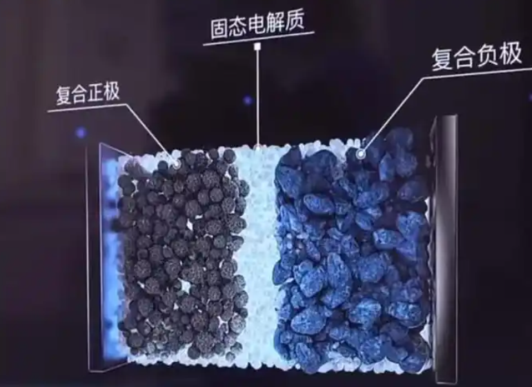
Modeling strategy for the solid electrolyte cell
I assume isothermal operation, continuous homogeneous layers, negligible in-plane transport, and linear elastic material behavior. The solid electrolyte cell is represented by three regions: positive electrode, solid polymer electrolyte, and negative electrode. The positive and negative electrodes store lithium, while the solid polymer electrolyte conducts lithium ions. Axial pressure is applied along the thickness direction. In-plane strain is constrained, and the thickness-direction stress is set by the external nominal pressure. The model couples lithium transport, interfacial reaction kinetics, mechanical stress, and pressure-dependent contact state.
The lithium transport in the positive and negative electrodes is described by
$$ \frac{\partial c_k}{\partial t}+\frac{\partial j_k}{\partial x}=0,\quad k=p,n $$
$$ j_k=-D_k\left(1-\frac{c_k}{c_k^{\max}}\right)\frac{\partial c_k}{\partial x}-\frac{D_k c_k}{RT}\Omega_k\frac{\partial \sigma_k}{\partial x} $$
Here, \(c_k\) is the lithium concentration, \(c_k^{\max}\) is the maximum host concentration, \(D_k\) is the diffusion coefficient, \(\Omega_k\) is the partial molar volume, \(\sigma_k\) is the hydrostatic stress, R is the gas constant, and T is temperature. The stress term in the flux expression allows mechanical stress to influence lithium transport. This coupling is important for a solid electrolyte cell because stress gradients can alter the chemical potential of lithium and therefore modify diffusion.
The solid polymer electrolyte uses a modified Nernst-Planck description:
$$ \frac{\partial c_e}{\partial t}+\frac{\partial j_e}{\partial x}=0 $$
$$ j_e=-D_e\left(\frac{\partial c_e}{\partial x}-\frac{c_e\Omega_e}{RT}\frac{\partial \sigma_e}{\partial x}\right) $$
where the effective diffusion coefficient and partial molar volume are
$$ D_e=\frac{2D_+D_-}{D_++D_-} $$
$$ \Omega_e=\Omega_++\Omega_- $$
The ionic current in the solid polymer electrolyte satisfies charge conservation:
$$ \frac{\partial i_e}{\partial x}=0 $$
$$ i_e=-\frac{F D_e(D_+-D_-)}{D_++D_-}\frac{\partial c_e}{\partial x}-\frac{F^2D_e c_e}{RT}\frac{\partial \Phi_e}{\partial x}+\frac{F D_e c_e}{RT}(\Omega_+-\Omega_-)\frac{\partial \sigma_e}{\partial x} $$
At each electrode-electrolyte interface, I use Butler-Volmer kinetics. For a solid electrolyte cell, the interfacial reaction current depends on the contact state because the effective reaction area is not equal to the nominal area. I write the general form as
$$ i_k=i_{k,0}\left[\exp\left(\frac{\alpha_k F\eta_k}{RT}\right)-\exp\left(-\frac{(1-\alpha_k)F\eta_k}{RT}\right)\right] $$
For the representative case with symmetric charge-transfer coefficients, this becomes
$$ i_k=2i_{k,0}\sinh\left(\frac{F\eta_k}{2RT}\right) $$
The reference exchange current density is a function of local lithium concentration, electrolyte lithium concentration, and reaction rate constant. The key contact modification is
$$ i_{p,0}^{\mathrm{eff}}=\gamma_{s1}i_{p,0} $$
$$ i_{n,0}^{\mathrm{eff}}=\gamma_{s2}i_{n,0} $$
where \(\gamma_{s1}\) and \(\gamma_{s2}\) are the contact factors at the positive electrode-solid electrolyte interface and the negative electrode-solid electrolyte interface, respectively. This is the first coupling path by which axial pressure affects the electrochemical response of the solid electrolyte cell. A higher pressure increases contact factor, enlarges the effective reaction area, raises the effective exchange current density, and lowers interfacial charge-transfer polarization.
The cell voltage is decomposed into five parts:
$$ V_{\mathrm{cell}}=V_{\mathrm{ref}}+V_{\mathrm{con}}+V_{\mathrm{str}}+V_{\mathrm{ove}}+V_{\mathrm{ele}} $$
This decomposition helps me separate concentration effects, stress effects, interfacial overpotential effects, and electrolyte potential effects. The reference voltage is fixed at 3.9 V. The concentration contribution depends on lithium concentrations at the reaction sites. The stress contribution depends on partial molar volumes and hydrostatic stresses. The overpotential contribution depends on the interfacial reaction kinetics. The electrolyte potential contribution is usually small in the present solid electrolyte cell parameters.
| Voltage component | Physical meaning | Expected pressure sensitivity |
|---|---|---|
| Reference voltage | Baseline thermodynamic potential | None |
| Concentration contribution | Lithium concentration difference at reaction sites | Weak direct sensitivity |
| Stress contribution | Chemical strain and hydrostatic stress | Small, corrective |
| Overpotential contribution | Interfacial charge-transfer polarization | Strong, dominant |
| Electrolyte potential contribution | Ionic potential drop in electrolyte | Small in this study |
Mechanical response and contact mechanics
The mechanical field in the solid electrolyte cell follows equilibrium:
$$ \nabla\cdot\sigma+b=0 $$
I assume zero in-plane strain, \(\varepsilon_{yy}=\varepsilon_{zz}=0\), and thickness-direction stress \(\sigma_{xx}=-P\), where P is the nominal axial pressure. The total strain is the sum of elastic strain and chemical strain:
$$ \varepsilon=\varepsilon^{\mathrm{elas}}+\varepsilon^{\mathrm{chem}} $$
The chemical strain is related to concentration change through partial molar volume. For the positive electrode, solid polymer electrolyte, and negative electrode, the thickness-direction strain can be expressed in the same general form:
$$ \varepsilon_k=\frac{(1+\nu_k)(1-2\nu_k)}{E_k}\frac{P}{3}+\frac{1}{3}\Omega_k(c_k-c_k^0)-\frac{\nu_k}{1-\nu_k}\varepsilon_k^{\mathrm{chem}} $$
Here, \(E_k\) is Young’s modulus, \(\nu_k\) is Poisson’s ratio, and \(c_k^0\) is the initial concentration. The total thickness change is obtained by integrating the strains of all layers:
$$ \Delta l=l_p\varepsilon_p+l_e\varepsilon_e+l_n\varepsilon_n $$
The maximum thickness variation H is defined as the difference between the maximum and minimum total thickness during a charge-discharge cycle:
$$ H(P)=\max_t l(P,t)-\min_t l(P,t) $$
For contact, I use a pressure-dependent contact factor. The real contact area A is usually smaller than the nominal area A0. I define
$$ \gamma=\frac{A}{A_0} $$
Based on Persson contact theory, the contact factor is computed from the rough-surface power spectrum:
$$ \gamma=\frac{1}{\sigma_0}\int_{q_L}^{\infty}\frac{4}{3}E^*qC(q)\operatorname{erf}\left(\frac{q}{2}\sqrt{\frac{2}{\pi}\frac{1}{\xi}}\right)dq $$
The equivalent modulus is
$$ \frac{1}{E^*}=\frac{1-\nu_1^2}{E_1}+\frac{1-\nu_2^2}{E_2} $$
The power spectrum is represented as
$$ C(q)=10^m q^I $$
The lower wavevector and the magnification factor are
$$ q_L=\frac{2\pi}{\sqrt{A_0}} $$
$$ \xi=\frac{A_0}{4Dt} $$
I treat the positive electrode-solid electrolyte interface as a film-type interface and the negative electrode-solid electrolyte interface as a bulk-type interface. The roughness parameters m and I are therefore different for the two interfaces. This is physically reasonable because the negative electrode has a more pronounced particulate morphology, while the positive electrode is a denser film.
The coupling from contact to mechanics is introduced by assuming that the nominal axial pressure is carried mainly by the real contact area. Thus, the effective elastic stress at the interface is amplified by \(1/\gamma\). The effective interfacial stress is written as the sum of an elastic bearing term and a chemical strain term:
$$ \sigma_{k,s}^{\mathrm{eff}}=\sigma_{k,s}^{\mathrm{elas}}+\sigma_{k,s}^{\mathrm{chem}} $$
For example, at the positive electrode-solid electrolyte interface,
$$ \sigma_{p,s1}^{\mathrm{eff}}=\frac{1}{3}\frac{P}{\gamma_{s1}}+\frac{E_p}{3(1-\nu_p)}\frac{\Omega_p}{3}(c_p-c_p^0)-\frac{\nu_p}{1-\nu_p}\sigma_{p,s1}^{\mathrm{chem}} $$
The exact algebraic form is less important than the coupling logic: as contact factor decreases, the elastic bearing term increases; as pressure increases, the elastic bearing term increases; as lithium concentration changes, the chemical stress term evolves. The interfacial stress difference is defined as
$$ \Delta\sigma_{s1}^{\mathrm{eff}}=\sigma_{p,s1}^{\mathrm{eff}}-\sigma_{e,s1}^{\mathrm{eff}} $$
$$ \Delta\sigma_{s2}^{\mathrm{eff}}=\sigma_{n,s2}^{\mathrm{eff}}-\sigma_{e,s2}^{\mathrm{eff}} $$
These stress differences measure mechanical mismatch across the solid-solid interfaces. In a solid electrolyte cell, a large stress difference is undesirable because it indicates that the two sides of the interface deform differently and may promote local damage, contact loss, or delamination under cycling.
| Model feature | Function in this work | Importance for solid electrolyte cell pressure optimization |
|---|---|---|
| Lithium transport with stress coupling | Resolves concentration and stress effects on flux | Captures chemical strain and diffusion-migration interaction |
| Butler-Volmer kinetics | Describes interfacial charge transfer | Links contact state to interfacial polarization |
| Persson contact factor | Quantifies real contact area under pressure | Provides pressure-dependent reaction area |
| Effective interfacial stress | Amplifies elastic bearing by contact factor | Represents local load concentration |
| Interfacial stress difference | Measures mechanical mismatch | Acts as a high-pressure penalty |
Parameterization and numerical solution
I solve the coupled system with a fully coupled solver and a sparse direct linear solver. The relative tolerance is 0.005, and the tolerance factor is 0.1. For pressure sweeps, I use a step of 0.3 MPa below 4 MPa and 1 MPa above 4 MPa. The temperature is 300 K, and the reference concentration is 1 mol/m3. The solid electrolyte cell is charged at 1 A/m2 to 4.03 V and then discharged at the same current density until SOC reaches 0.05. This protocol is used consistently unless otherwise stated.
| Parameter | Positive electrode | Solid polymer electrolyte | Negative electrode |
|---|---|---|---|
| Thickness (nm) | 550 | 2000 | 200 |
| Maximum concentration (mol/m3) | 23300 | 1500 | 30555 |
| Initial concentration (mol/m3) | 22135 | 1200 | 1527.75 |
| Reaction rate constant (m2.5 mol-0.5 s-1) | 1.53e-11 | – | 5.03e-11 |
| Diffusion coefficient (m2/s) | 1.76e-15 | 2.5e-13 for cation, 3e-13 for anion | 8e-14 |
| Partial molar volume (m3/mol) | 1.92e-6 | 3.95e-6 for cation, 1.46e-4 for anion | 4.17e-6 |
| Charge-transfer coefficient | 0.5 | – | 0.5 |
| Young’s modulus (GPa) | 70 | 0.5 | 10 |
| Poisson’s ratio | 0.20 | 0.40 | 0.30 |
Validation logic
I validate the electrochemical part by setting both contact factors equal to one and comparing the terminal voltage versus SOC curve with a published benchmark solid electrolyte cell. The voltage plateau, SOC range, and high-SOC voltage variation agree well. The coefficient of determination is 0.9931, and the maximum absolute voltage error is 0.0310 V. This indicates that the baseline electrochemical behavior is captured reliably.
I also examine the impedance scaling with contact area. In the small-overpotential limit, the interfacial impedance is inversely proportional to the effective exchange current density. Since I introduce the contact factor linearly into the exchange current density, the interfacial impedance scales approximately as \(1/\gamma\). The area coefficient is therefore about -1. Published experimental area coefficients are typically in the range -1.13 to -1.05. The agreement in order and sensitivity supports the coupling form used in this solid electrolyte cell model.
For the pressure sensitivity of charge-transfer resistance, I define a normalized resistance:
$$ R_{\mathrm{norm}}(P)=\frac{R_{\mathrm{ct}}(P)-R_{\mathrm{ct}}(P_0)}{R_{\mathrm{ct}}(P_0)} $$
The total charge-transfer resistance is approximated as
$$ R_{\mathrm{ct}}=\frac{RT}{F}\left(\frac{1}{i_{p,0}^{\mathrm{eff}}}+\frac{1}{i_{n,0}^{\mathrm{eff}}}\right) $$
For a representative pressure change, the model prediction is close to published experimental values. This further supports the pressure-dependent contact model and its use in axial pressure window optimization for a solid electrolyte cell.
Effect of axial pressure on contact state
I first evaluate how axial pressure changes the contact factor at both interfaces. As pressure increases, the contact factor increases rapidly at low pressure and then approaches saturation at higher pressure. The positive electrode-solid electrolyte interface reaches nearly complete contact at a relatively low pressure, around 4 MPa. The negative electrode-solid electrolyte interface recovers more slowly and requires a higher pressure to approach full contact. This difference arises from the different roughness parameters assigned to film-type and bulk-type interfaces.
| Pressure range | Positive interface contact | Negative interface contact | Interpretation |
|---|---|---|---|
| Very low pressure | Incomplete | Strongly incomplete | Reaction area limited, high polarization |
| Low to medium pressure | Rapidly improving | Moderately improving | Capacity utilization increases |
| Medium pressure | Nearly saturated | Still improving | Marginal electrochemical gain decreases |
| High pressure | Saturated | Close to saturation | Contact benefit small, mechanical cost continues |
The contact factor directly modifies the effective exchange current density. When contact is poor, the nominal current must be carried by a smaller real area, so the local current density is higher. This increases the interfacial overpotential required to sustain the same total current. The result is a lower terminal voltage, earlier voltage cutoff, and lower usable capacity. When contact improves, the effective reaction area increases, the overpotential decreases, and the solid electrolyte cell can operate over a wider SOC range.
Electrochemical response under axial pressure
I plot the discharge voltage versus capacity for different contact factors. As the contact factor increases, the discharge curve shifts toward higher voltage and higher capacity. This shift is caused by reduced interfacial polarization. In a solid electrolyte cell, the usable capacity is not only determined by the intrinsic storage capacity of the electrodes but also by the ability of the interfaces to transfer charge at a sufficient rate. If the interface is contact-limited, the cell reaches the cutoff voltage before the electrodes are fully utilized.
The voltage decomposition shows that the overpotential contribution is the most pressure-sensitive component. The concentration contribution varies mainly with SOC and is only weakly affected by pressure. The stress contribution increases with SOC and is somewhat larger at higher pressure, but its magnitude remains on the order of tens of millivolts. Therefore, the main electrochemical benefit of axial pressure in a solid electrolyte cell is the reduction of interfacial overpotential, not a direct change in concentration or stress voltage terms.
| Voltage component | Response to increasing axial pressure | Contribution to capacity improvement |
|---|---|---|
| Concentration contribution | Weak direct change | Secondary |
| Stress contribution | Slight increase with pressure and SOC | Corrective, small |
| Overpotential contribution | Strong decrease as contact improves | Dominant |
| Electrolyte potential contribution | Very small | Negligible in this study |
At low pressure, the overpotential contribution is large because the effective reaction area is small. As pressure increases, the contact factor increases, the effective exchange current density increases, and the overpotential contribution falls. The relative share of the concentration contribution therefore increases. This does not mean that pressure directly enhances concentration effects; it means that the overpotential penalty is removed, so the concentration term becomes a larger fraction of the remaining voltage components.
At higher SOC, the overpotential contribution is larger than at lower SOC. This suggests that interfacial polarization has a stronger influence on the solid electrolyte cell when the electrodes are more delithiated or lithiated, depending on the direction of operation. The stress contribution also increases with SOC because chemical strain becomes larger as lithium concentration changes. However, the stress term remains much smaller than the concentration and overpotential terms. The primary electrochemical conclusion is that axial pressure improves capacity utilization by improving contact and reducing interfacial polarization, but the benefit decreases as pressure rises.
Mechanical response under axial pressure
I next examine the stress distribution along the thickness direction. The stress state differs among the positive electrode, solid polymer electrolyte, and negative electrode. As SOC increases, the positive electrode tends to develop larger tensile stress, while the negative electrode develops larger compressive stress. The solid polymer electrolyte experiences smaller stress amplitudes than the electrodes. This behavior is caused by differences in elastic modulus, partial molar volume, and concentration change among the layers.
At the same SOC, the direct effect of axial pressure on the layer stress distribution is relatively limited. When pressure increases from 0.1 MPa to 1 MPa, the stress profiles change only slightly. When pressure increases further to 10 MPa or 50 MPa, the compressive stress in the solid polymer electrolyte and negative electrode increases modestly, while the tensile stress in the positive electrode changes little. This means that the internal stress of a solid electrolyte cell is not controlled by external pressure alone. It is determined by the combination of external pressure, concentration-induced chemical strain, and material property mismatch.
Axial pressure also changes the accessible SOC range. At low pressure, the solid electrolyte cell cannot reach high SOC because interfacial polarization causes early voltage cutoff. At higher pressure, improved contact and lower overpotential allow the cell to operate at higher SOC. At high SOC, chemical strain is larger, so the stress difference between layers becomes more pronounced. Therefore, axial pressure indirectly increases mechanical stress by extending the operating SOC range.
| Quantity | Low pressure | Medium pressure | High pressure |
|---|---|---|---|
| Interfacial contact | Poor | Good | Near saturated |
| Interfacial overpotential | High | Reduced | Low |
| Usable SOC range | Narrow | Wide | Wide but saturating |
| Layer stress amplitude | Lower due to narrow SOC | Moderate | Higher due to high SOC |
| Interfacial stress difference | Lower in absolute value | Increasing | High |
| Pressurization cost | Low | Moderate | High |
The maximum interfacial stress difference increases with axial pressure. The increase is steep at low pressure and becomes gentler at higher pressure. This behavior has two causes. First, when contact is incomplete, the nominal pressure is carried mainly by the real contact area. The effective bearing stress is therefore amplified. As contact improves, this amplification is reduced. Second, higher pressure extends the SOC range, allowing larger chemical strain at high SOC. These two effects oppose each other in terms of local amplification but do not cancel the overall increase. The result is a monotonic but sublinear increase in maximum interfacial stress difference with pressure.
The positive electrode-solid electrolyte interface has a larger maximum stress difference than the negative electrode-solid electrolyte interface in this model. This indicates that the positive side is the more critical interface for mechanical mismatch under the present material parameters. For a solid electrolyte cell, this finding suggests that pressure optimization should not only consider the weaker contact interface but also the interface with the larger stress mismatch. In this case, the negative interface limits contact recovery at low pressure, while the positive interface limits mechanical risk at high pressure.
The maximum thickness variation H increases with pressure and then flattens. At low pressure, H increases noticeably because the solid electrolyte cell can access a wider SOC range as contact improves. At high pressure, contact improvement saturates, and the additional increase in SOC range is small. The absolute magnitude of H remains in the nanometer range for the thin-film geometry considered here. Relative to the total thickness, this variation is small. Therefore, overall thickness breathing is useful as an indicator of operating deformation, but it is not the main factor that limits the upper pressure bound. The maximum interfacial stress difference is a more meaningful mechanical penalty for high pressure.
Numerical reliability and parameter sensitivity
I perform mesh independence tests, time-step independence tests, and roughness parameter sensitivity studies. For mesh independence, I compare five mesh schemes. The maximum voltage difference among schemes is 0.274 mV, and the maximum difference in positive interfacial stress difference at 10 MPa is 0.111 MPa. These differences are very small relative to the quantities of interest. I therefore use a relatively coarse uniform mesh for the pressure sweep.
| Mesh scheme | Positive electrode elements | Solid electrolyte elements | Negative electrode elements | Total elements |
|---|---|---|---|---|
| M1 | 14 | 18 | 10 | 42 |
| M2 | 21 | 27 | 15 | 63 |
| M3 | 35 | 45 | 25 | 105 |
| M4 | 70 | 90 | 50 | 210 |
| M5 | 140 | 180 | 100 | 420 |
For time-step independence, I compare maximum time steps of 2 s, 1 s, 0.5 s, 0.25 s, and 0.125 s. The maximum voltage difference is 0.53 mV, and the interfacial stress difference is nearly identical across time steps. I therefore select 2 s as a balance between accuracy and computational cost.
| Time-step scheme | Maximum time step |
|---|---|
| T1 | 2 s |
| T2 | 1 s |
| T3 | 0.5 s |
| T4 | 0.25 s |
| T5 | 0.125 s |
For roughness sensitivity, I vary the contact parameters m and I over a wide range. When the interface becomes rougher, the contact factor recovers more slowly with pressure. The low-pressure charge-discharge curves differ more strongly among roughness cases, while the medium- and high-pressure curves are similar. The qualitative conclusion remains unchanged: increasing pressure enlarges the operating SOC range of the solid electrolyte cell. The maximum interfacial stress difference also increases with pressure for all roughness cases, although the absolute values differ.
| Case | Positive interface m | Negative interface m | Positive interface I | Negative interface I |
|---|---|---|---|---|
| Base | -2.77 | -3.08 | -9.35 | -6.61 |
| R1 | -2.67 | -2.98 | -10.35 | -7.61 |
| R2 | -2.72 | -3.03 | -9.85 | -7.11 |
| R3 | -2.82 | -3.13 | -8.85 | -6.11 |
| R4 | -2.87 | -3.18 | -8.35 | -5.61 |
Multi-criteria evaluation of the axial pressure window
I now formulate the pressure optimization problem. The goal is to select an axial pressure that improves the solid electrolyte cell without allowing mechanical risk and pressurization cost to grow without bound. I use four normalized indicators: usable areal capacity, minimum interfacial contact factor, maximum interfacial stress difference, and pressurization cost. The first two are benefit-type indicators, and the last two are cost-type indicators.
The usable areal capacity is calculated from the discharge current density and cutoff time:
$$ Q(P)=\frac{i_{\mathrm{app}}t_{\mathrm{cut}}(P)}{3600} $$
The normalized capacity indicator is
$$ Q_n(P)=\frac{Q(P)-Q_{\min}}{Q_{\max}-Q_{\min}} $$
The minimum contact factor is the worse of the two interfaces:
$$ \gamma_{\min}(P)=\min\left(\gamma_{s1}(P),\gamma_{s2}(P)\right) $$
Its normalized form is
$$ \gamma_{\min,n}(P)=\frac{\gamma_{\min}(P)-\gamma_{\min,\min}}{\gamma_{\min,\max}-\gamma_{\min,\min}} $$
The maximum interfacial stress difference is
$$ S(P)=\max\left(|\Delta\sigma_{s1}^{\mathrm{eff}}|,|\Delta\sigma_{s2}^{\mathrm{eff}}|\right) $$
and its normalized form is
$$ S_n(P)=\frac{S(P)-S_{\min}}{S_{\max}-S_{\min}} $$
The normalized pressurization cost is
$$ P_n(P)=\frac{P-P_{\min}}{P_{\max}-P_{\min}} $$
I then define a composite loss function:
$$ J(P)=\omega_Q\left[1-Q_n(P)\right]^2+\omega_\gamma\left[1-\gamma_{\min,n}(P)\right]^2+\omega_S S_n(P)+\omega_P P_n(P) $$
The optimal pressure for a given weight set is
$$ P^*=\arg\min_{P_{\min}\le P\le P_{\max}} J(P) $$
I choose three representative weight schemes: a performance-priority scheme, a balanced scheme, and a conservative scheme. The performance-priority scheme emphasizes capacity and contact. The balanced scheme considers capacity, contact, stress difference, and pressurization cost with moderate weights. The conservative scheme places more weight on stress difference and pressurization cost.
| Scheme | Capacity weight | Contact weight | Stress-difference weight | Pressure-cost weight |
|---|---|---|---|---|
| Performance priority | 0.35 | 0.40 | 0.15 | 0.10 |
| Balanced | 0.30 | 0.35 | 0.20 | 0.15 |
| Conservative | 0.25 | 0.30 | 0.25 | 0.20 |
Because the objective function is computed from the full coupled model, I avoid an explicit analytical gradient. I use particle swarm optimization with direct calls to the model. Each particle position is a candidate axial pressure. The velocity and position updates are
$$ v_i^{k+1}=\omega v_i^k+c_1r_1\left(p_i^k-P_i^k\right)+c_2r_2\left(g^k-P_i^k\right) $$
$$ P_i^{k+1}=P_i^k+v_i^{k+1} $$
I use 15 particles and 9 iterations. The inertia weight is 0.65, the individual and group learning factors are both 1.45, and the velocity limit is 8 MPa. After the swarm search, I perform a local scan around the best pressure to refine the result.
To verify that the result is not algorithm-specific, I also use a deterministic method. I combine a full-range coarse scan with one-dimensional bounded optimization on candidate intervals. I use shape-preserving piecewise cubic Hermite interpolation for the normalized capacity, contact, and stress indicators, while the pressure cost remains analytical. The coarse scan uses a maximum interval of 1 MPa. Candidate minima are refined with a bounded one-dimensional optimizer. The convergence tolerance is 1e-3 MPa, the maximum number of iterations is 200, and the maximum number of objective evaluations is 500.
| Optimization scheme | Particle swarm result | Deterministic result | Difference |
|---|---|---|---|
| Performance priority | 15.8 MPa | 15.7 MPa | 0.1 MPa |
| Balanced | 12.2 MPa | 12.4 MPa | 0.2 MPa |
| Conservative | 10.0 MPa | 9.8 MPa | 0.2 MPa |
The two methods agree within 0.2 MPa for all three schemes. This gives me confidence that the pressure window is not an artifact of a particular search algorithm. The particle swarm method is convenient because it does not require an interpolation surrogate, but the deterministic method confirms the result.
Optimal pressure window and trade-off behavior
I examine the normalized indicators as functions of pressure. The normalized capacity and contact factor both increase with pressure, but their growth rates differ. Capacity rises quickly at low pressure and flattens after about 10 MPa. Contact factor continues to increase over a wider pressure range, especially for the weaker negative interface. The normalized stress difference and pressure cost also increase with pressure. The pressure cost increases almost linearly, while the stress difference increases rapidly at low pressure and then more slowly.
| Indicator | Trend with pressure | Role in optimization |
|---|---|---|
| Normalized capacity | Increases, then saturates | Benefit |
| Normalized minimum contact factor | Increases, slower saturation | Benefit |
| Normalized maximum stress difference | Increases, sublinear at high pressure | Cost |
| Normalized pressurization cost | Increases linearly | Cost |
For the balanced scheme, the composite loss function reaches a minimum near 12.2 MPa. At lower pressure, the capacity and contact penalties dominate. At higher pressure, the stress-difference and pressure-cost penalties dominate. The minimum therefore represents a compromise between electrochemical benefit and mechanical or engineering cost.
I also compute the contributions of each term in the balanced loss function. At low pressure, the capacity term and contact term are large. As pressure increases, both decrease. The stress-difference term and pressure-cost term increase. The total loss first falls and then rises, producing a clear minimum. This behavior is characteristic of axial pressure optimization for a solid electrolyte cell: pressure is necessary for contact, but additional pressure eventually becomes counterproductive when mechanical and pressurization penalties are included.
| Scheme | Usable areal capacity (Ah/m2) | Minimum contact factor | Maximum stress difference (MPa) | Pressure (MPa) |
|---|---|---|---|---|
| Performance priority | 0.1368 | 0.8079 | 579.25 | 15.8 |
| Balanced | 0.1342 | 0.7471 | 574.93 | 12.2 |
| Conservative | 0.1316 | 0.6971 | 569.51 | 10.0 |
The performance-priority scheme selects a higher pressure because it values capacity and contact more strongly. The conservative scheme selects a lower pressure because it penalizes stress difference and pressure cost more strongly. The balanced scheme selects an intermediate pressure. The fact that all three schemes fall within a relatively narrow band indicates that the useful pressure window for this solid electrolyte cell is not extremely wide. The trade-off optimum is therefore better described as a window rather than a single universal pressure.
I further define marginal electrochemical benefit and marginal mechanical or pressure cost:
$$ B(P)=\frac{Q_n(P)+\gamma_{\min,n}(P)}{2} $$
$$ C(P)=\frac{S_n(P)+P_n(P)}{2} $$
The marginal changes for a 1 MPa pressure increment are
$$ \Delta B=B(P+\Delta P)-B(P) $$
$$ \Delta C=C(P+\Delta P)-C(P) $$
At low pressure, the marginal benefit is larger than the marginal cost. As pressure increases, the marginal benefit falls rapidly. At medium pressure, the marginal benefit and marginal cost become comparable. At high pressure, the marginal cost exceeds the marginal benefit. The pressure at which the two curves are closest is consistent with the balanced optimum. This marginal analysis supports the interpretation that the optimal pressure window is where the solid electrolyte cell still gains meaningful electrochemical performance but has not yet accumulated excessive mechanical and pressurization penalties.
| Pressure region | Marginal benefit versus cost | Recommended interpretation |
|---|---|---|
| Below about 10 MPa | Benefit usually exceeds cost | Under-pressurized, contact-limited |
| About 10 to 16 MPa | Benefit and cost are comparable | Trade-off window |
| Above about 16 MPa | Cost exceeds benefit | Over-pressurized for marginal electrochemical gain |
Based on the multi-criteria optimization and marginal analysis, I identify a trade-off axial pressure window of 10.0 to 15.8 MPa for the material system, ideal layered structure, and isothermal conditions considered here. The balanced scheme gives a trade-off optimum of 12.2 MPa. This window is not a universal design rule for every solid electrolyte cell, but it is a model-based recommendation for the present parameter set and evaluation criteria.
Robustness of the pressure window
I test the robustness of the pressure window in several ways. First, I randomly sample weight combinations from broad ranges. The weights satisfy the constraint that they sum to one. I obtain 5000 valid samples and compute the optimal pressure for each. The optimal pressures are concentrated in the medium-pressure range. The 5th, 25th, 50th, 75th, and 95th percentiles are 7.12 MPa, 9.10 MPa, 11.10 MPa, 13.81 MPa, and 17.92 MPa, respectively. The median is 11.10 MPa, which is close to the balanced optimum. About 63.56 percent of the samples fall within the trade-off window. This indicates that the window is not a fragile result of one weight choice.
| Statistic | Optimal pressure (MPa) |
|---|---|
| 5th percentile | 7.12 |
| 25th percentile | 9.10 |
| Median | 11.10 |
| 75th percentile | 13.81 |
| 95th percentile | 17.92 |
Second, I vary the normalization intervals. The original interval is 0.1 to 50 MPa. When the upper bound is extended by 20 percent to 60 MPa, the optimal window becomes 10.8 to 17.1 MPa. When the interval is set to the 5th to 95th percentile range, 2.6 to 47.5 MPa, the window becomes 11.8 to 17.9 MPa. Although the endpoints shift, the windows overlap strongly with the original window. The pressure range remains medium.
| Normalization interval | Trade-off pressure window |
|---|---|
| Original: 0.1 to 50 MPa | 10.0 to 15.8 MPa |
| Upper bound extended by 20 percent | 10.8 to 17.1 MPa |
| 5th to 95th percentile | 11.8 to 17.9 MPa |
Third, I vary the loss function form. I compare the original form, a fully quadratic form, a normalized Huber form with threshold 0.5, and an exponential form. The original form gives 10.0 to 15.8 MPa. The fully quadratic form gives 11.5 to 16.7 MPa. The Huber form gives 12.8 to 17.5 MPa. The exponential form gives 11.0 to 18.6 MPa. All windows remain in the medium-pressure range and overlap with the original window. This suggests that the qualitative pressure window is not highly sensitive to the exact mathematical form of the loss function.
For the Huber form, I use
$$ J(P)=\omega_Q H(1-Q_n(P))+\omega_\gamma H(1-\gamma_{\min,n}(P))+\omega_S H(S_n(P))+\omega_P H(P_n(P)) $$
with
$$ H(x)=
\begin{cases}
\frac{2}{3}x^2, & 0\le x\le 0.5,\\
\frac{4}{3}x-\frac{1}{3}, & 0.5<x\le $$="" 1.=""
For the exponential form, I use
$$ J(P)=\omega_Q E(1-Q_n(P))+\omega_\gamma E(1-\gamma_{\min,n}(P))+\omega_S E(S_n(P))+\omega_P E(P_n(P)) $$
with
$$ E(x)=\frac{e^{2x}-1}{e^{2x}+1} $$
| Loss function form | Trade-off pressure window |
|---|---|
| Original form | 10.0 to 15.8 MPa |
| Fully quadratic form | 11.5 to 16.7 MPa |
| Normalized Huber form | 12.8 to 17.5 MPa |
| Exponential form | 11.0 to 18.6 MPa |
Fourth, I vary the charge and discharge current density. Lower current densities shift the optimal window slightly toward lower pressure. The original current density of 1 A/m2 gives 10.0 to 15.8 MPa. A lower current density of 0.135 A/m2 gives 8.8 to 14.0 MPa. A higher but still moderate current density of 0.744 A/m2 gives 9.9 to 15.8 MPa. The changes are modest, and all windows remain in the medium-pressure range. This supports the stability of the pressure window with respect to current-density variations in the tested range.
| Charge and discharge current density | Trade-off pressure window |
|---|---|
| 1 A/m2 | 10.0 to 15.8 MPa |
| 0.135 A/m2 | 8.8 to 14.0 MPa |
| 0.270 A/m2 | 9.3 to 14.9 MPa |
| 0.406 A/m2 | 9.6 to 15.4 MPa |
| 0.541 A/m2 | 9.8 to 15.6 MPa |
| 0.744 A/m2 | 9.9 to 15.8 MPa |
Engineering load implication for the solid electrolyte cell
For an engineering perspective, I convert the optimal pressure window into total preload force for a representative large-format pouch solid electrolyte cell. I use an effective cell area of 120 mm by 80 mm, which is 0.0096 m2. The preload force is
$$ F=pA $$
For the pressure window of 10.0 to 15.8 MPa, the total preload force is approximately 96.0 to 151.7 kN. The balanced optimum of 12.2 MPa corresponds to about 117.1 kN. This is a high but plausible load for a well-designed fixture. It also shows that pressure optimization has direct structural consequences for the solid electrolyte cell module. The end plates, fasteners, and compression frames must be designed to maintain this load without excessive deflection or stress concentration.
| Pressure | Preload force for 120 mm x 80 mm cell |
|---|---|
| 10.0 MPa | 96.0 kN |
| 12.2 MPa | 117.1 kN |
| 15.8 MPa | 151.7 kN |
The recommended pressure window is consistent with typical high-pressure fixtures reported for large-format solid electrolyte cell testing. A uniform pressure distribution requires careful design of the compression fixture. If the fixture is stiff and well aligned, the pressure distribution can be reasonably uniform. If not, local pressure concentrations can increase the mechanical risk beyond what the average pressure suggests. Therefore, the pressure window I identify should be understood as a nominal average pressure for an ideal layered solid electrolyte cell. In a real module, the distribution of pressure must be verified.
Discussion of coupling mechanisms
The most important coupling in this study is the pressure-contact-kinetics path. Axial pressure changes the real contact area. The real contact area changes the effective exchange current density. The effective exchange current density changes the interfacial overpotential. The interfacial overpotential changes the terminal voltage and the accessible SOC range. Finally, the accessible SOC range changes the chemical strain and the internal stress state. This chain explains why axial pressure has both electrochemical and mechanical consequences in a solid electrolyte cell.
A second coupling is the pressure-contact-mechanics path. The nominal pressure is carried by the real contact area. When contact is poor, the local bearing stress is amplified. This amplification contributes to the effective interfacial stress. As pressure increases, contact improves and amplification decreases, but the nominal pressure itself increases. The net result is that the maximum interfacial stress difference increases with pressure, although the rate of increase slows at high pressure.
A third coupling is the concentration-stress-transport path. Lithium concentration changes cause chemical strain, which changes stress. Stress gradients appear in the chemical potential and therefore influence lithium flux. This path is present even without external pressure, but axial pressure modifies it by changing the accessible SOC range and the mechanical boundary condition.
| Coupling path | Primary variables | Main consequence for solid electrolyte cell |
|---|---|---|
| Pressure-contact-kinetics | P, contact factor, exchange current density, overpotential | Controls capacity utilization and voltage |
| Pressure-contact-mechanics | P, contact factor, effective bearing stress, stress difference | Controls interfacial mechanical risk |
| Concentration-stress-transport | c, chemical strain, stress, flux | Controls internal stress evolution and diffusion |
| SOC-pressure-mechanics | Accessible SOC, chemical strain, layer stress | Indirectly increases high-pressure mechanical penalty |
This multi-path coupling is why a single-indicator optimization is inadequate. If I optimize only capacity, I will choose a high pressure. If I optimize only stress difference, I will choose a low pressure. If I optimize only contact factor, I will again choose a high pressure because contact continues to improve. The balanced loss function is necessary to capture the fact that the solid electrolyte cell has an interior optimum.
Limitations and extension paths
The present model is one-dimensional and assumes an ideal layered structure. It does not explicitly resolve particle-level contact, crack initiation, void formation, delamination, or interfacial damage evolution. These mechanisms become more important as pressure and cycle number increase. A more complete model of a solid electrolyte cell would include cohesive zone laws, fracture energy, interfacial strength, and damage variables. It would also include the mechanical behavior of the fixture, end plates, and compression frame, because pressure uniformity and structural compliance affect the actual pressure seen by the cell.
The model is isothermal. Temperature affects ionic conductivity, reaction kinetics, and mechanical properties. In an automotive solid electrolyte cell, temperature gradients and high-rate operation may change the optimal pressure window. Future work should include temperature as a state variable and examine high-rate, overcharge, overdischarge, and abnormal pressure conditions.
The pressure window obtained here is specific to the material parameters and ideal geometry used in the simulation. Different solid electrolytes, electrode materials, porosities, particle sizes, and surface roughness values will shift the window. Therefore, the window should be treated as a model-based design target, not as a universal constant. Experimental validation on solid electrolyte cell prototypes and modules is necessary to refine the parameters and confirm the predicted trade-off.
Conclusions
I have developed a coupled electro-chemo-mechanical model for a solid electrolyte cell under axial pressure. The model includes pressure-dependent solid-solid contact, interfacial reaction kinetics, lithium transport, chemical strain, and interfacial stress difference. I use the model to evaluate axial pressure as a multi-criteria design variable rather than a fixed operating condition.
The main conclusions are as follows.
First, axial pressure improves the solid electrolyte cell by increasing the real contact area at the electrode-solid electrolyte interfaces. The improved contact raises the effective exchange current density, lowers interfacial overpotential, and increases usable areal capacity. The positive electrode-solid electrolyte interface reaches good contact at relatively low pressure, while the negative electrode-solid electrolyte interface requires higher pressure. The electrochemical benefit of pressure is strong at low pressure and decreases at medium and high pressure.
Second, axial pressure also increases mechanical and engineering penalties. The maximum interfacial stress difference increases with pressure because the nominal load increases and because the accessible SOC range expands. The positive electrode-solid electrolyte interface shows a larger stress difference than the negative interface in this material system. The maximum thickness variation increases at low pressure and then flattens, but its absolute magnitude is small compared with the interfacial stress difference. Therefore, interfacial stress difference is the more important upper-bound constraint.
Third, the multi-criteria optimization shows that a balanced axial pressure window exists. For the present material system, ideal layered structure, and isothermal conditions, the trade-off pressure window is 10.0 to 15.8 MPa. The balanced scheme gives an optimum of 12.2 MPa. Performance-priority, balanced, and conservative schemes give optima of 15.8 MPa, 12.2 MPa, and 10.0 MPa, respectively. These values are close to those obtained by a deterministic optimization method, with differences no larger than 0.2 MPa.
Fourth, the pressure window is robust to reasonable variations in weights, normalization intervals, loss function forms, and current densities. Random weight sampling places the median optimum at 11.10 MPa and about 63.56 percent of samples within the trade-off window. Varying the normalization interval and loss function shifts the window endpoints but does not move the window out of the medium-pressure range. Varying the current density by a factor of several changes the window only modestly.
Fifth, the optimal pressure window has practical engineering implications. For a large-format solid electrolyte cell with an effective area of 120 mm by 80 mm, the preload force corresponding to 10.0 to 15.8 MPa is approximately 96.0 to 151.7 kN. This load is manageable with a stiff and well-aligned compression fixture, but it requires careful design of end plates, fasteners, and pressure distribution. The nominal pressure window should not be confused with a guarantee of uniform local pressure in a real solid electrolyte cell module.
Overall, I conclude that axial pressure optimization for a solid electrolyte cell should be based on a coupled electrochemical-mechanical evaluation. Pressure is necessary to maintain solid-solid contact and to reduce interfacial polarization, but excessive pressure increases interfacial stress mismatch and pressurization cost without proportional electrochemical gain. The balanced window identified here provides a method-level reference for pressure regulation and interfacial reliability analysis of solid electrolyte cells, especially for multilayer integrated cells intended for automotive applications.
Future work should extend this framework to rough interfaces with damage evolution, interfacial debonding, and local contact failure. It should also include module-level constraints such as end-plate stiffness, structural mass, pressure uniformity, and thermal effects. Experimental measurement of interfacial stress and contact area in operating solid electrolyte cells would help validate and refine the pressure window. With these extensions, the multi-criteria pressure optimization method can support the design of safer, higher-energy, and more reliable solid electrolyte cell systems.