
In the field of renewable energy integration, the design and optimization of hybrid power systems, particularly those combining hydroelectric and solar photovoltaic (PV) generation, have garnered significant attention. My research focuses on determining the optimal tilt angle for solar panels within such hydro-solar hybrid systems, especially when facing non-uniform electrical load demands and seasonal variations in hydroelectric generation capacity. Traditional methods for calculating the optimal tilt angle of solar panels often assume a uniformly distributed annual load, leading to recommendations that maximize solar radiation capture during the month of weakest insolation. However, this approach is inadequate for systems where load demand fluctuates monthly and where hydropower availability is significantly higher during wet seasons compared to dry seasons. The improper tilt angle can result in substantial energy waste during periods of surplus or critical energy deficits during shortages, unnecessarily increasing storage costs and reducing system reliability. Therefore, a refined methodology is essential to align solar panel output more closely with the temporal profile of net load—the load demand minus the available hydropower. This article presents a comprehensive model and analysis, employing a least squares optimization technique to determine the tilt angle that best balances seasonal solar energy harvest with the specific consumption and generation patterns of a hydro-solar hybrid system.
The core of the analysis begins with accurately modeling the amount of solar radiation received on an inclined surface where the solar panels are mounted. The total solar radiation incident on a horizontal surface, denoted as \( H \), comprises the beam (direct) component \( H_b \) and the diffuse (sky-scattered) component \( H_d \):
$$ H = H_b + H_d $$
For a south-facing solar panel array in the Northern Hemisphere (or north-facing in the Southern Hemisphere) tilted at an angle \( \beta \) from the horizontal, the total incident radiation \( H_T \) includes three parts: the beam radiation on the tilted surface \( H_{bT} \), the diffuse radiation on the tilted surface \( H_{dT} \), and the radiation reflected from the ground onto the surface \( H_{rT} \). Thus,
$$ H_T = H_{bT} + H_{dT} + H_{rT} $$
These components can be related to the horizontal radiation quantities through geometrical and empirical factors:
$$ H_T = H_b R_b + H_d R_d + \rho H R_g $$
Here, \( R_b \) is the beam radiation factor, \( R_d \) is the diffuse radiation factor, \( \rho \) is the ground reflectivity (albedo, typically assumed as 0.2 for ordinary ground), and \( R_g \) is the factor for ground-reflected radiation. For a surface tilted towards the equator, these factors are calculated as follows. The beam radiation factor \( R_b \) is the ratio of beam radiation on the tilted surface to that on the horizontal surface:
$$ R_b = \frac{\cos(\phi – \beta) \cos \delta \sin \omega_s + \frac{\pi}{180} \omega_s \sin(\phi – \beta) \sin \delta}{\cos \phi \cos \delta \sin \omega_0 + \frac{\pi}{180} \omega_0 \sin \phi \sin \delta} $$
In this equation, \( \phi \) represents the local latitude, \( \beta \) is the tilt angle of the solar panels, \( \delta \) is the solar declination angle, \( \omega_s \) is the sunset hour angle for the tilted surface, and \( \omega_0 \) is the sunset hour angle for the horizontal surface. The solar declination \( \delta \) in degrees for the \( n \)-th day of the year is given by:
$$ \delta = 23.45 \sin\left( \frac{360 (284 + n)}{365} \right) $$
The sunset hour angle for the horizontal surface, \( \omega_0 \), is:
$$ \omega_0 = \cos^{-1}(-\tan \phi \tan \delta) $$
The sunset hour angle for the tilted surface, \( \omega_s \), is the minimum of the horizontal sunset angle and the angle specific to the tilt:
$$ \omega_s = \min\left( \cos^{-1}(-\tan \phi \tan \delta), \cos^{-1}(-\tan(\phi – \beta) \tan \delta) \right) $$
The diffuse radiation factor \( R_d \) accounts for the anisotropic distribution of diffuse sky radiation. A common model expresses it using the ratio of beam to total horizontal radiation, \( K_b = H_b / H \), and a clearness index \( K_t \). However, for many practical calculations, a simplified form using an isotropic model combined with a circumsolar component is used. A widely adopted formulation is:
$$ R_d = K_b R_b + (1 – K_b) \left( \frac{1 + \cos \beta}{2} \right) $$
In this context, \( K_b \) is the monthly average ratio of beam radiation on a horizontal surface to the total horizontal radiation. The ground-reflected radiation factor \( R_g \) assumes isotropic reflection and is simply:
$$ R_g = \frac{1 – \cos \beta}{2} $$
Combining these, the total daily radiation on a tilted surface for day \( n \) can be expressed as:
$$ H_{T_n} = H_n \left[ K_b R_{b_n} + (1 – K_b) R_{d_n} + \rho R_g \right] $$
By summing these daily values, the monthly total radiation on the tilted solar panels, \( H_{TM}(m, \beta) \), for month \( m \) and tilt angle \( \beta \), and the annual total \( H_T(\beta) \) can be computed. This model forms the foundational physics for assessing the energy yield of solar panels at different installation angles.
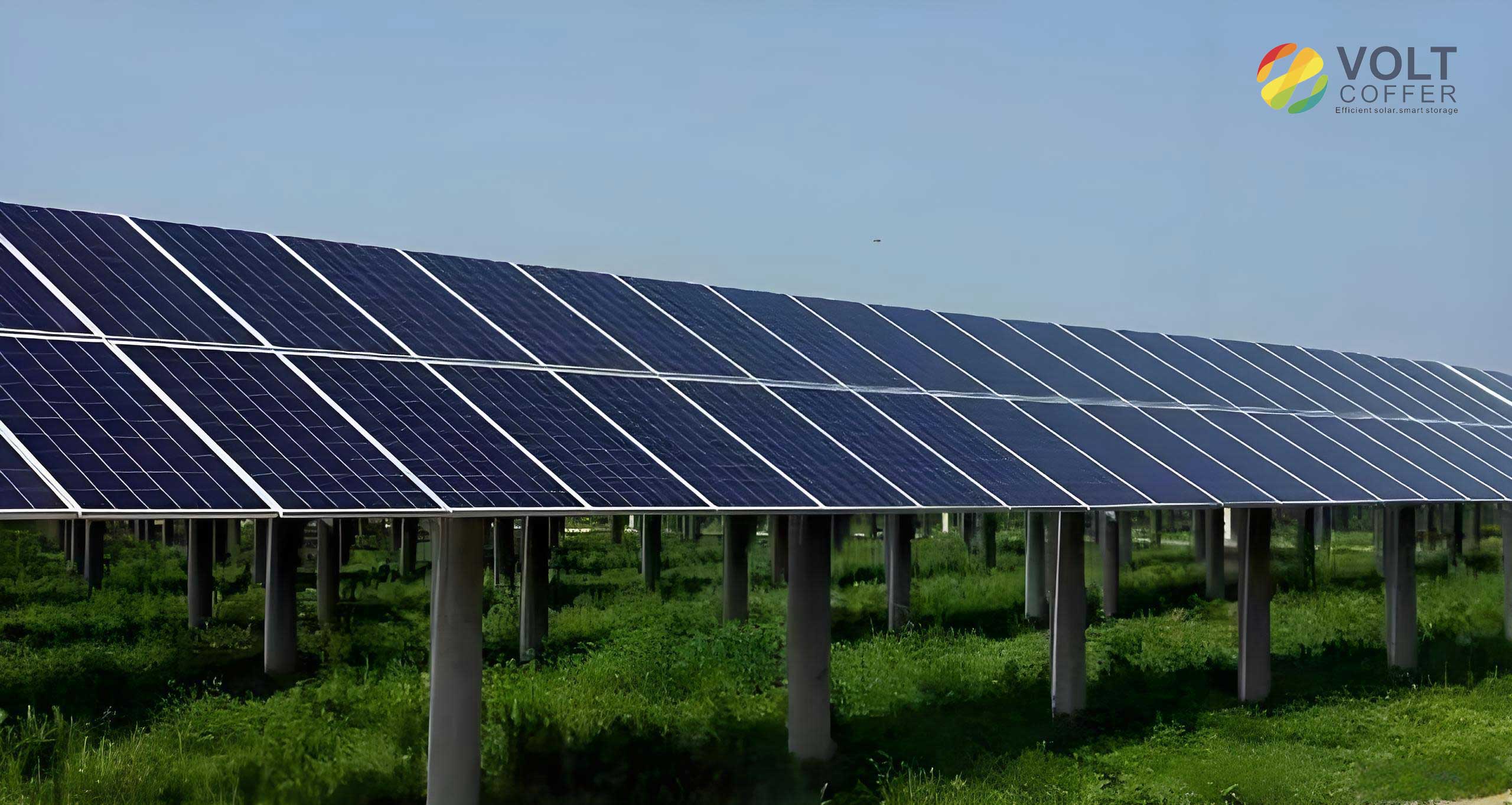
To determine the optimal tilt angle for solar panels in a hybrid system context, one must consider not just the maximization of annual solar input, but its temporal alignment with the net load. The net load for any given month is the electrical load demand that must be met after accounting for the available hydroelectric generation. Let \( L(m) \) be the average load demand for month \( m \), and \( W(m) \) be the average available hydroelectric generation for that month. The net load \( N(m) \) is then \( N(m) = L(m) – W(m) \). In an ideal scenario, the energy generated by the solar panels \( S(m, \beta) \) would exactly match \( N(m) \) for each month. The solar generation is proportional to the incident radiation on the panels, so \( S(m, \beta) = \eta \cdot A \cdot H_{TM}(m, \beta) \), where \( \eta \) is the system efficiency and \( A \) is the total area of the solar panels. For optimization relative to tilt angle, the constants \( \eta \) and \( A \) can be omitted when comparing proportions.
Therefore, the problem reduces to finding the tilt angle \( \beta \) that makes the profile of monthly solar radiation \( H_{TM}(m, \beta) \) most closely match the profile of the net load \( N(m) \). Since both profiles are seasonal, a least squares minimization approach is adopted. We define the following normalized monthly ratios:
- Solar Radiation Ratio: \( S_R(m, \beta) = \frac{H_{TM}(m, \beta)}{\sum_{m=1}^{12} H_{TM}(m, \beta)} \) – the fraction of annual solar radiation received in month \( m \) at tilt \( \beta \).
- Load Ratio: \( L_R(m) = \frac{L(m)}{\sum_{m=1}^{12} L(m)} \) – the fraction of annual load consumed in month \( m \).
- Hydropower Generation Ratio: \( W_R(m) = \frac{W(m)}{\sum_{m=1}^{12} W(m)} \) – the fraction of annual hydropower generated in month \( m \).
The ideal target profile for the solar panels to complement is the Net Load Ratio, which can be approximated by the difference \( L_R(m) – W_R(m) \), normalized to a comparable scale. However, for direct least squares fitting, we seek to minimize the discrepancy between the solar input and the required complement. We define a monthly difference or error term \( E(m, \beta) \):
$$ E(m, \beta) = L_R(m) – W_R(m) – S_R(m, \beta) $$
This represents how much the solar contribution, relative to its annual total, deviates from the relative net load requirement. The optimal tilt angle \( \beta_{opt} \) is the one that minimizes the sum of squared errors over all months:
$$ \text{Minimize: } J(\beta) = \sum_{m=1}^{12} \left[ E(m, \beta) \right]^2 $$
Alternatively, one could also minimize the sum of squared deviations of \( S_R(m, \beta) \) from a scaled version of \( (L_R(m) – W_R(m)) \). The core principle is to align the seasonal shape of solar energy capture with the seasonal shape of energy deficit after hydropower contribution. This method ensures that during months with lower hydropower output (e.g., dry season) and potentially higher load, the tilt of the solar panels is adjusted to capture relatively more sun, and vice-versa during high-hydro months.
To illustrate the application of this methodology, let’s consider a representative case study for a location at a latitude of approximately 36° N, resembling the conditions of a region with a large hydro-solar hybrid plant. The key input data required are: daily horizontal solar radiation \( H_n \), the beam fraction \( K_b \), monthly load data \( L(m) \), and monthly hydropower capacity factor or generation \( W(m) \). For this analysis, typical meteorological year data or satellite-derived solar radiation data (e.g., from NASA’s SSE database) can be used. The ground albedo \( \rho \) is taken as 0.2. The beam fraction \( K_b \) is often derived from atmospheric clarity data; for this region, an annual average value of 0.6 is assumed, meaning 60% of horizontal radiation is direct beam.
The first computational step is to calculate the monthly total solar radiation on surfaces with various tilt angles, from 0° (horizontal) to 60° in suitable increments, using the model equations and a tool like MATLAB or Python. The table below presents the calculated monthly total radiation \( H_{TM}(m, \beta) \) (in arbitrary energy units, e.g., kWh/m²) and the annual total \( H_T(\beta) \) for tilt angles from 0° to 60° in 10° steps, based on synthesized data representative of the location.
| Month | β=0° | β=10° | β=20° | β=30° | β=40° | β=50° | β=60° |
|---|---|---|---|---|---|---|---|
| January | 66.65 | 83.89 | 99.23 | 112.22 | 122.45 | 129.61 | 133.50 |
| February | 83.22 | 97.95 | 110.53 | 120.57 | 127.78 | 131.93 | 132.90 |
| March | 138.74 | 152.60 | 163.21 | 170.25 | 173.50 | 172.87 | 168.37 |
| April | 173.08 | 179.88 | 183.11 | 182.66 | 178.50 | 170.78 | 159.74 |
| May | 172.20 | 172.24 | 169.33 | 163.44 | 154.70 | 143.37 | 129.85 |
| June | 130.42 | 128.18 | 123.97 | 117.79 | 109.77 | 100.15 | 89.27 |
| July | 142.74 | 141.41 | 137.78 | 131.85 | 123.75 | 113.71 | 102.10 |
| August | 150.72 | 154.17 | 154.71 | 152.26 | 146.89 | 138.75 | 128.11 |
| September | 113.28 | 121.74 | 127.65 | 130.83 | 131.18 | 128.70 | 123.44 |
| October | 103.93 | 119.52 | 132.50 | 142.50 | 149.20 | 152.40 | 152.01 |
| November | 78.66 | 97.14 | 113.44 | 127.07 | 137.62 | 144.75 | 148.27 |
| December | 71.75 | 92.18 | 110.51 | 126.19 | 138.74 | 147.77 | 153.02 |
| Annual Total \( H_T(\beta) \) | 1425.39 | 1540.88 | 1625.98 | 1677.63 | 1694.08 | 1674.82 | 1620.57 |
From Table 1, we observe that the maximum annual radiation is received at a tilt angle around 40° (1694.08 units), which is slightly higher than the latitude of 36°. This is often referred to as the “maximum annual yield” angle for solar panels. However, this angle may not be optimal for our hybrid system context. Next, we compute the solar radiation ratio \( S_R(m, \beta) \) for each angle, as shown in Table 2.
| Month | β=0° | β=10° | β=20° | β=30° | β=40° | β=50° | β=60° |
|---|---|---|---|---|---|---|---|
| Jan | 0.0468 | 0.0544 | 0.0610 | 0.0669 | 0.0723 | 0.0774 | 0.0824 |
| Feb | 0.0584 | 0.0636 | 0.0680 | 0.0719 | 0.0754 | 0.0788 | 0.0820 |
| Mar | 0.0973 | 0.0990 | 0.1003 | 0.1015 | 0.1024 | 0.1032 | 0.1039 |
| Apr | 0.1214 | 0.1167 | 0.1126 | 0.1089 | 0.1054 | 0.1020 | 0.0986 |
| May | 0.1208 | 0.1118 | 0.1041 | 0.0974 | 0.0913 | 0.0856 | 0.0801 |
| Jun | 0.0915 | 0.0832 | 0.0762 | 0.0702 | 0.0648 | 0.0598 | 0.0551 |
| Jul | 0.1001 | 0.0918 | 0.0847 | 0.0786 | 0.0731 | 0.0679 | 0.0630 |
| Aug | 0.1057 | 0.1000 | 0.0951 | 0.0908 | 0.0867 | 0.0829 | 0.0791 |
| Sep | 0.0795 | 0.0790 | 0.0785 | 0.0780 | 0.0774 | 0.0769 | 0.0762 |
| Oct | 0.0729 | 0.0776 | 0.0815 | 0.0850 | 0.0881 | 0.0910 | 0.0938 |
| Nov | 0.0552 | 0.0630 | 0.0697 | 0.0757 | 0.0812 | 0.0865 | 0.0915 |
| Dec | 0.0503 | 0.0598 | 0.0679 | 0.0752 | 0.0819 | 0.0883 | 0.0944 |
The load data is synthesized based on typical regional consumption patterns, showing higher demand in winter and summer months due to heating and cooling needs. The monthly load ratios \( L_R(m) \) are calculated from a multi-year average, resulting in the following values:
| Month | Jan | Feb | Mar | Apr | May | Jun | Jul | Aug | Sep | Oct | Nov | Dec |
|---|---|---|---|---|---|---|---|---|---|---|---|---|
| \( L_R(m) \) | 0.092 | 0.078 | 0.088 | 0.083 | 0.087 | 0.088 | 0.098 | 0.101 | 0.088 | 0.086 | 0.090 | 0.099 |
For hydropower, we assume a significant seasonal variation: a dry season from December to March where generation is at 80% of the plant’s rated capacity, and a wet season for the rest of the year where it operates at 100% capacity. Normalizing the monthly generation to form the ratio \( W_R(m) \), we get:
| Month | Jan | Feb | Mar | Apr | May | Jun | Jul | Aug | Sep | Oct | Nov | Dec |
|---|---|---|---|---|---|---|---|---|---|---|---|---|
| \( W_R(m) \) | 0.0714 | 0.0714 | 0.0714 | 0.0893 | 0.0893 | 0.0893 | 0.0893 | 0.0893 | 0.0893 | 0.0893 | 0.0893 | 0.0714 |
The net load ratio target, \( L_R(m) – W_R(m) \), is then computed. For example, in January: \( 0.092 – 0.0714 = 0.0206 \). The complete set of monthly target values \( T(m) = L_R(m) – W_R(m) \) is:
| Month | Jan | Feb | Mar | Apr | May | Jun | Jul | Aug | Sep | Oct | Nov | Dec |
|---|---|---|---|---|---|---|---|---|---|---|---|---|
| \( T(m) \) | 0.0206 | 0.0066 | 0.0166 | -0.0063 | -0.0023 | -0.0013 | 0.0087 | 0.0117 | -0.0013 | -0.0033 | 0.0007 | 0.0276 |
Note that negative values indicate months where hydropower alone exceeds the load, so solar contribution could ideally be lower. The objective is to find \( \beta \) such that \( S_R(m, \beta) \) approximates \( T(m) \) as closely as possible. However, since \( T(m) \) can be negative and \( S_R(m, \beta) \) is always positive, we primarily aim to match the relative seasonal pattern. In practice, we minimize the sum of squared differences \( E(m, \beta) = T(m) – S_R(m, \beta) \). The sum of squared errors \( J(\beta) = \sum_{m=1}^{12} E(m, \beta)^2 \) is calculated for each tilt angle. The results for the coarse 10° increments are:
| Tilt Angle β | 0° | 10° | 20° | 30° | 40° | 50° | 60° |
|---|---|---|---|---|---|---|---|
| \( J(\beta) \) | 0.0184 | 0.0069 | 0.0047 | 0.0033 | 0.0026 | 0.0024 | 0.0025 |
Table 6 shows that the error decreases as the tilt angle increases from 0° to around 50°, where it reaches a minimum of 0.0024, and then slightly increases at 60°. To pinpoint the optimum, a finer resolution calculation was performed around 50°. The analysis reveals that the minimum sum of squared errors occurs at a tilt angle of approximately 52°. This is notably different from the angle that maximizes annual radiation (around 40°). Therefore, for this non-uniform load and hydro-generation scenario, the optimal installation angle for the solar panels is 52°, not 40°.
The physical interpretation is clear: at a steeper tilt of 52°, the solar panels capture more sunlight during the winter months (December, January, February) when the sun is lower in the sky and, critically, when hydropower is at its lower capacity (80%) and load is relatively high. Conversely, during summer months, especially June and July, when hydropower is abundant and load, while potentially high, is partly met by hydro, the steeper tilt reduces the relative solar contribution because the panels are less optimally oriented for the high summer sun. This seasonal balancing act enhances the overall reliability of the hybrid system and can reduce the required battery storage capacity, as the solar output better complements the hydro resource throughout the year.
It is important to discuss the sensitivity of this result to input parameters. The optimal tilt angle for solar panels depends on the specific shapes of the load and hydro generation profiles. If the load profile were flatter or the hydro variation less pronounced, the optimal angle might shift closer to the maximum radiation angle. Similarly, different geographic locations with different solar regimes (e.g., more diffuse radiation) would yield different optimums. The beam fraction \( K_b \) also plays a role; regions with higher diffuse radiation might see a different relationship between tilt and seasonal distribution. Furthermore, the economic aspect, such as the cost of solar panels versus storage or the value of energy at different times, could be integrated into a more sophisticated optimization that weighs monthly errors by economic factors. However, the least squares method on normalized ratios provides a robust and straightforward engineering approach for initial design.
Another consideration is the potential for dual-axis or seasonal adjustment of the solar panels. While fixed-tilt systems are simpler and cheaper, the significant difference between the maximum-yield angle (40°) and the system-optimum angle (52°) suggests that a seasonally adjustable tilt could harvest even more energy while maintaining good complementarity. For instance, one could set a steeper tilt in winter and a shallower tilt in summer. However, the cost and complexity of tracking mechanisms must be justified by the increased system benefits. For many large-scale hybrid installations, fixed-tilt solar panels remain the standard, making the choice of a single, year-round optimal angle crucial.
In conclusion, determining the optimal tilt angle for solar panels in a hydro-solar hybrid power generation system under non-uniform load conditions requires a holistic approach that goes beyond simply maximizing annual solar insolation. By modeling the solar radiation on tilted surfaces and applying a least squares optimization to align the seasonal profile of solar energy capture with the seasonal profile of net load (load minus hydropower), a more suitable tilt angle can be identified. In the representative case studied, the optimum was found to be 52°, which is steeper than the latitude-plus-15° rule of thumb or the maximum annual radiation angle of 40°. This angle better utilizes the solar panels to offset energy deficits during low-hydro months, thereby improving the stability and economic efficiency of the hybrid system. This methodology provides a valuable framework for engineers designing such integrated renewable energy systems, ensuring that the solar panel array is configured not just for maximum harvest, but for maximum utility within the specific generation and consumption context. Future work could expand this model to incorporate detailed economic optimization, different solar radiation models, and the effects of temperature on solar panel efficiency, further refining the guidance for installing solar panels in complex hybrid energy environments.