
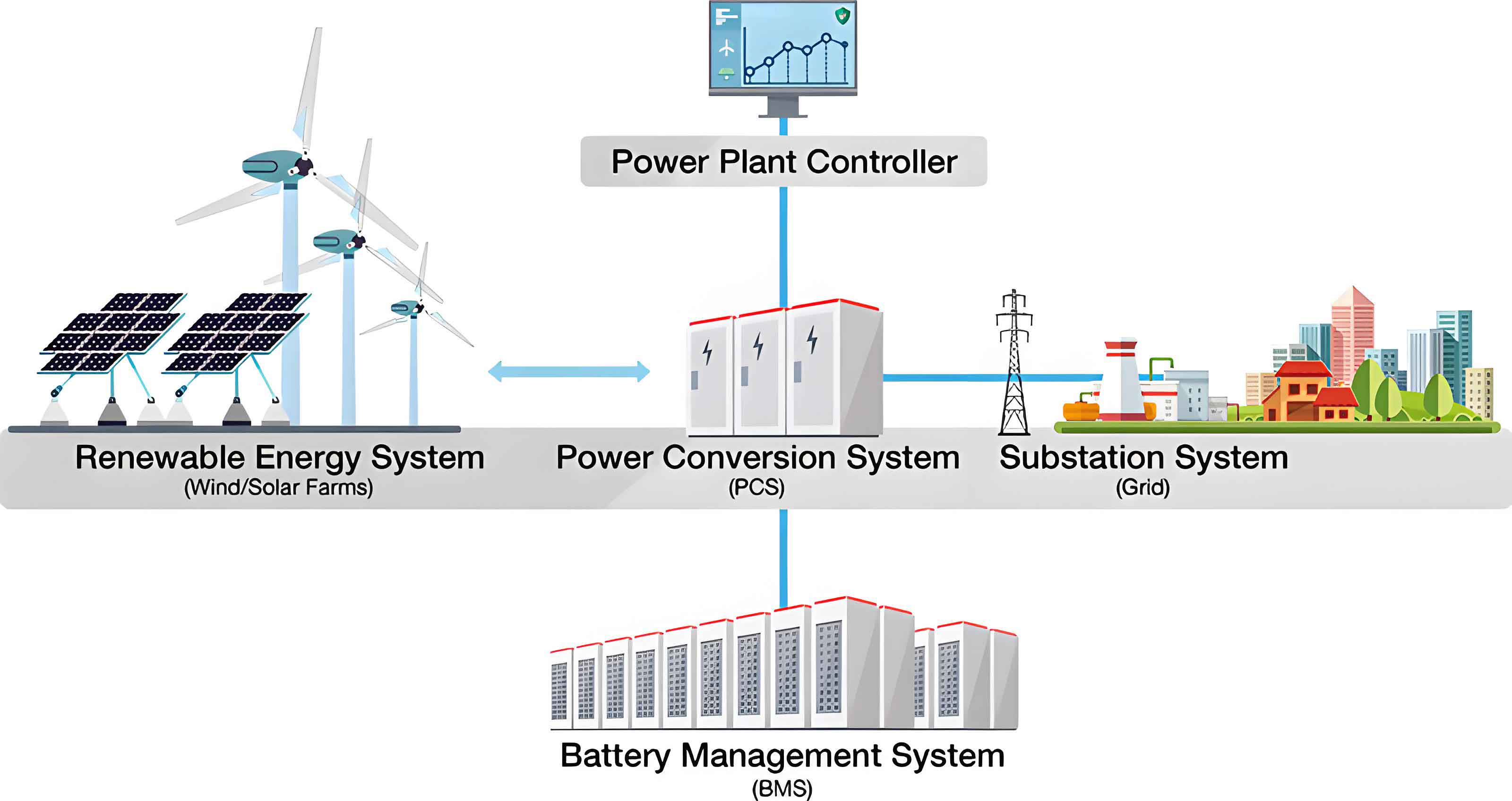
The global push towards carbon peaking and carbon neutrality goals is driving a profound transformation of the energy landscape, significantly increasing the share of clean, renewable sources. In this context, the battery energy storage system has emerged as a critical enabler, providing essential support for grid stability, load balancing, and the integration of intermittent renewables like solar and wind. As a core component of modern battery energy storage system installations, the lithium-ion battery’s operational state is paramount for safety, efficiency, and longevity. Among various state parameters, the State of Charge (SOC)—defined as the ratio of remaining capacity to maximum available capacity—is fundamental. It provides a crucial reference for the Battery Management System (BMS) to formulate charge/discharge strategies, preventing hazardous over-charge or over-discharge conditions. However, SOC cannot be measured directly and must be inferred indirectly from measurable parameters such as voltage, current, and temperature.
Current SOC estimation methods can be broadly categorized into two groups: model-based methods and data-driven methods. Model-based approaches, such as the Ampere-hour (Ah) integration and the Open-Circuit Voltage (OCV) method, rely on physical or electrochemical models of the battery. While simple, the Ah integration method suffers from accumulated error due to current sensor drift and unknown initial conditions. The OCV method offers good accuracy but requires the battery to be at rest for a long period to reach equilibrium, making it unsuitable for real-time applications in a dynamic battery energy storage system. Kalman Filter variants, which are also model-based, provide robust estimates but their accuracy is highly sensitive to the precision of the battery model and noise statistics.
Data-driven methods, particularly neural networks, have gained substantial attention as they can learn the complex, non-linear relationship between measurable inputs and SOC without requiring an explicit, precise physical model. Traditional Back-Propagation (BP) neural networks are commonly used but are prone to getting trapped in local minima and can be sensitive to initial weight values. To overcome these limitations and achieve higher estimation accuracy for enhanced battery energy storage system management, we propose a novel data-driven framework based on a Modified Probabilistic Neural Network (MPNN). The MPNN innovatively combines a probabilistic layer for robust feature extraction with a compensation mechanism that optimizes the inference process, leading to superior global search capability and fitting accuracy compared to conventional networks.
Fundamentals of SOC Estimation
The SOC of a lithium-ion battery is formally defined as:
$$ S_{\text{LiB}} = \frac{Q_c}{Q_{\text{max}}} \times 100\% $$
where $Q_c$ is the current remaining charge and $Q_{\text{max}}$ is the maximum charge capacity. A common equivalent circuit model used to describe battery dynamics is the first-order RC model, which includes an open-circuit voltage source $V_1$, an ohmic internal resistor $R_1$, and an RC parallel network ($R_2$, $C$) representing polarization dynamics. The terminal voltage $V_0$ and current $I$ are the primary measurable outputs and input, respectively.
Deriving SOC from this model involves solving differential equations and is complicated by factors like hysteresis, aging, and temperature effects. From a mathematical perspective, SOC is a non-linear function of the measurable quantities: $S_{\text{LiB}} = f(V_0, I, T, \dots)$. The core challenge is to approximate this unknown function $f(\cdot)$ with high fidelity. Our MPNN approach tackles this as a supervised learning problem, mapping time-series data of voltage, current, and temperature directly to the corresponding SOC value, thus bypassing the need for intricate model identification and proving highly adaptable for diverse battery energy storage system configurations.
Architecture of the Modified Probabilistic Neural Network (MPNN)
The proposed MPNN features an eight-layer hierarchical structure designed to progressively transform raw input data into a precise SOC estimate. The architecture is summarized in the table below and detailed in the subsequent sections.
| Layer Number | Layer Name | Primary Function | Key Parameters/Operations |
|---|---|---|---|
| 1 | Input Layer | Accepts measurable parameters (V, I, T, etc.). | Number of nodes $m$ equals number of inputs. |
| 2 | Normalization Layer | Scales all inputs to a [0,1] range. | Min-max normalization. |
| 3 | Probability Layer | Transforms inputs into probability space using radial basis functions. | Centers $c_{kj}^3$, widths $b_{kj}^3$, Gaussian RBF. |
| 4 | Threshold Layer | Filters out weak probability signals to focus on salient features. | Predefined threshold $th$. |
| 5 | Fuzzy Rule Layer | Aggregates thresholded probabilities through weighted summation. | Weights $w_{kj}^4$. |
| 6 | Compensation Layer | Introduces compensatory degrees of freedom to optimize the inference mechanism. | Compensation factor $c_j$. |
| 7 | Output Layer | Produces the normalized SOC estimate. | Output weights $w_j^7$. |
| 8 | Virtual Layer | Denormalizes the output to obtain the final SOC value. | Reverse of Layer 2 operation. |
1. Input and Normalization Layers
The network accepts $m$ measurable inputs, denoted as $X_k$ (e.g., $X_1$=Voltage, $X_2$=Current, $X_3$=Temperature). The input layer simply passes these values:
$$ f^1_k = x^1_k = X_k, \quad k=1,2,\dots,m $$
The normalization layer then scales each input to a standard range [0, 1] to ensure stable and efficient training:
$$ f^2_k = \frac{x^2_k – x^2_{k,\text{min}}}{x^2_{k,\text{max}} – x^2_{k,\text{min}}}, \quad \text{where } x^2_k = f^1_k $$
Here, $x^2_{k,\text{min}}$ and $x^2_{k,\text{max}}$ are the minimum and maximum values of the $k$-th input variable observed in the training dataset.
2. Probability and Threshold Layers
This is the first core innovation. The probability layer contains $n$ pattern nodes for each input, utilizing a Gaussian Radial Basis Function (RBF) to convert the normalized inputs into probability measures. This approach provides a smoother, more robust transformation than direct linear weighting.
$$ f^3_{kj} = \exp\left( -\frac{(x^3_{kj} – c^3_{kj})^2}{2 (b^3_{kj})^2} \right), \quad x^3_{kj}=f^2_k, \quad k=1,\dots,m; j=1,\dots,n $$
$c^3_{kj}$ and $b^3_{kj}$ are the center and width of the $j$-th Gaussian node for the $k$-th input. The threshold layer then acts as a filter:
$$ f^4_{kj} = x^4_{kj} =
\begin{cases}
0, & \text{if } f^3_{kj} \leq th \\
f^3_{kj}, & \text{if } f^3_{kj} > th
\end{cases}
$$
This step suppresses negligible probability values, enhancing the network’s focus on the most relevant features and improving computational efficiency for the battery energy storage system BMS.
3. Fuzzy Rule, Compensation, and Output Layers
The fuzzy rule layer aggregates the filtered probabilities. Each of its $n$ nodes computes a weighted sum of all thresholded outputs associated with the same pattern index $j$ across all inputs:
$$ f^5_j = x^5_j = \sum_{k=1}^{m} w^4_{kj} f^4_{kj}, \quad j=1,\dots,n $$
where $w^4_{kj} = \exp(wi^4_{kj}) > 0$ are positive weights ensuring proper aggregation.
The compensation layer is the second core innovation. It introduces adaptive compensatory factors $c_j$ to refine the inference mechanism from the fuzzy rule layer, providing additional degrees of freedom to better capture the complex SOC dynamics.
$$ f^6_j = x^6_j = (x^5_j)^{1 – c_j} \cdot \left( \frac{c_j}{m} \right), \quad j=1,\dots,n $$
$$ \text{with } c_j = \frac{1}{1 + \exp(-ci_j)} \in (0,1) $$
The compensation factor $c_j$ adjusts the influence of the fuzzy rule output. When $c_j \rightarrow 0$, the output relies mainly on $x^5_j$; when $c_j \rightarrow 1$, it introduces a constant bias, allowing the network to learn more complex mappings essential for accurate battery energy storage system state estimation.
The output layer generates the final normalized SOC estimate by linearly combining the compensated values:
$$ \hat{S}_{\text{LiB, norm}} = f^7 = \sum_{j=1}^{n} w^7_j x^7_j, \quad \text{where } x^7_j = f^6_j $$
The virtual layer performs denormalization to obtain the actual SOC estimate:
$$ \hat{S}_{\text{LiB}} = \frac{f^7 \cdot (Q_{\text{max}} – Q_{\text{min}}) + Q_{\text{min}}}{Q_{\text{max}}} $$
where $Q_{\text{min}}$ is the minimum capacity value from the normalized training data range.
SOC Estimation Framework Based on MPNN
The implementation of MPNN for SOC estimation in a battery energy storage system involves a clear training and deployment pipeline. The process is as follows:
Step 1: Data Collection & Preprocessing. Historical operational data from the battery energy storage system, including voltage, current, temperature, and corresponding true SOC (calculated via high-precision laboratory methods like controlled Ah integration for training), is collected. The data is partitioned into training and testing sets.
Step 2: Network Initialization. Key parameters are initialized: RBF centers $c^3_{kj}$ are spaced evenly across [0,1], widths $b^3_{kj}$ are set to $1/n$, the threshold $th=0.001$, compensation factors $ci_j$ are set to 0, and weights $wi^4_{kj}$, $w^7_j$ are randomly initialized within a small range.
Step 3: Training Phase. The network is trained using gradient descent to minimize the loss function, defined as the Sum of Squared Errors (SSE) between the estimated SOC and the true SOC from the training data:
$$ E = \frac{1}{2} \sum_{i=1}^{N_{\text{train}}} e_i^2 = \frac{1}{2} \sum_{i=1}^{N_{\text{train}}} (S_{\text{LiB},i} – \hat{S}_{\text{LiB},i})^2 $$
The weights $wi^4_{kj}$ and $w^7_j$ are updated iteratively. The learning rules derived via backpropagation are:
$$ \Delta wi^4_{kj} = \eta_{wi^4} \cdot e_i \cdot \frac{Q_{\text{max}}-Q_{\text{min}}}{Q_{\text{max}}} \cdot w^7_j \cdot \left(1 – c_j + \frac{c_j}{m}\right) \cdot \frac{x^6_j}{x^5_j} \cdot f^4_{kj} \cdot w^4_{kj} $$
$$ \Delta w^7_j = \eta_{w^7} \cdot e_i \cdot \frac{Q_{\text{max}}-Q_{\text{min}}}{Q_{\text{max}}} \cdot x^7_j $$
where $\eta_{wi^4}$ and $\eta_{w^7}$ are the learning rates.
Step 4: Deployment/Testing Phase. Once trained, the MPNN model is fixed. Real-time or unseen test data from the battery energy storage system (voltage, current, temperature) is fed through the network’s forward pass (Layers 1 to 8) to generate instantaneous SOC estimates without requiring any battery model.
Simulation Results and Performance Analysis
To validate the proposed MPNN, extensive tests were conducted using publicly available datasets from the CALCE Battery Research Group for a 18650-20R lithium-ion battery (nominal capacity 2000 mAh). The performance was compared against a standard Fuzzy Neural Network (FNN) and a basic Probabilistic Neural Network (PNN). Two key metrics were employed: Mean Absolute Error (MAE) and Root Mean Square Error (RMSE).
$$ \text{MAE} (E_{MA}) = \frac{1}{N} \sum_{i=1}^{N} |e_i| $$
$$ \text{RMSE} (E_{RMS}) = \sqrt{ \frac{1}{N} \sum_{i=1}^{N} e_i^2 } $$
Test 1: Low Constant Current Charge/Discharge
The battery was charged at a constant 0.1A from 0% to 80% SOC and then discharged at 0.1A from 80% to 10% SOC. The MPNN estimates closely tracked the reference SOC. The estimation relative error remained consistently within ±1% throughout both charge and discharge cycles, demonstrating excellent accuracy under stable, low-rate conditions typical of some battery energy storage system operational phases.
Test 2: Dynamic Current Profile
A more realistic and challenging dynamic current profile, simulating variable charge/discharge loads in a real battery energy storage system, was applied. The SOC estimation results and relative errors are summarized below.
| Method | Description | Max Absolute Error | MAE ($E_{MA}$) | RMSE ($E_{RMS}$) |
|---|---|---|---|---|
| FNN | Standard Fuzzy Neural Network | > 3% | ~0.0025 | ~0.0070 |
| PNN | Basic Probabilistic Neural Network | < 3% | ~0.0021 | ~0.0045 |
| MPNN (Proposed) | Modified Probabilistic Neural Network | < 1% | ~0.0009 | ~0.0012 |
The proposed MPNN clearly outperformed both FNN and PNN, with its maximum error and average error metrics being significantly lower. This confirms that the integration of the probability layer and the compensation mechanism effectively enhances the network’s ability to learn the complex non-linear mapping under dynamic conditions.
Test 3: Robustness Across Different Temperatures
The performance of the three methods was further evaluated across a range of ambient temperatures (0°C to 50°C) using dynamic current profiles. Consistent performance across temperature variations is vital for a reliable battery energy storage system BMS deployed in diverse climates.
| Temperature (°C) | MAE ($E_{MA}$) | RMSE ($E_{RMS}$) | ||||
|---|---|---|---|---|---|---|
| FNN | PNN | MPNN | FNN | PNN | MPNN | |
| 0 | 0.0048 | 0.0041 | 0.0018 | 0.0098 | 0.0062 | 0.0022 |
| 10 | 0.0032 | 0.0030 | 0.0011 | 0.0077 | 0.0045 | 0.0014 |
| 20 | 0.0027 | 0.0026 | 0.0009 | 0.0072 | 0.0041 | 0.0012 |
| 25 | 0.0023 | 0.0021 | 0.0009 | 0.0069 | 0.0040 | 0.0012 |
| 30 | 0.0020 | 0.0018 | 0.0010 | 0.0064 | 0.0042 | 0.0011 |
| 40 | 0.0021 | 0.0019 | 0.0012 | 0.0065 | 0.0045 | 0.0013 |
| 50 | 0.0028 | 0.0024 | 0.0013 | 0.0068 | 0.0047 | 0.0015 |
The results unequivocally show that the MPNN maintains superior accuracy (lowest MAE and RMSE) across the entire temperature spectrum. While all methods see some performance variation with temperature, the MPNN’s error metrics are consistently about 50% or less than those of the PNN and FNN, proving its enhanced robustness. This makes it a highly suitable candidate for SOC estimation in real-world battery energy storage system applications that experience fluctuating environmental conditions.
Conclusion
Accurate State-of-Charge estimation is a cornerstone for the safe, efficient, and reliable operation of any lithium-ion battery energy storage system. To address the limitations of traditional model-based and basic data-driven methods, this work presented a novel Modified Probabilistic Neural Network (MPNN). The MPNN architecture innovatively merges a probability layer using Gaussian kernels with a flexible compensation mechanism. This combination enables the network to avoid local minima during training and achieve a highly accurate global approximation of the complex SOC function. Comprehensive validation tests under low constant-current, dynamic current, and varying temperature conditions demonstrated that the MPNN significantly outperforms standard Fuzzy Neural Networks and basic Probabilistic Neural Networks. The proposed method consistently achieved SOC estimation errors with MAE and RMSE below 1%, showcasing its precision, robustness, and strong potential for practical implementation in advanced battery management systems for grid-scale and commercial battery energy storage system deployments.