
In the context of the global “dual-carbon” strategy and the accelerated construction of new power systems, the penetration of renewable energy sources such as wind and photovoltaic power in microgrids continues to increase. However, the strong randomness and volatility of wind and solar power generation significantly raise the operational risks of microgrids, severely constraining system stability and the efficient integration of renewable energy. To address these challenges, I constructed a “source-storage-load” collaborative bi-level optimization model and proposed a multi-strategy Improved Beluga Whale Optimizer (IBWO) for solving this model, aiming to improve both the economic efficiency and stability of microgrid operations. The core research focus centers on the optimal design and operational scheduling of the energy storage system, which acts as the essential buffer for renewable energy fluctuations.
The energy storage system embodies diverse technological pathways, each exhibiting distinct characteristics in terms of power density, energy density, response speed, and applicable scenarios. Electrochemical batteries, exemplified by lithium-ion technology, dominate current applications due to rapid response and technical maturity, yet their cycle life and energy density pose limitations for long-duration storage. Conversely, hydrogen storage offers high energy density and extended storage periods, rendering it particularly suitable for seasonal or long-cycle compensation of renewable generation shortfalls. Mechanical storage, such as pumped hydro, requires specific geographical conditions that limit deployment flexibility. Recent research underscores the complementary advantages of integrating multiple storage technologies into a hybrid energy storage system, where batteries manage high-frequency power transients and hydrogen units handle low-frequency, long-duration energy balancing tasks. A comprehensive comparison of storage technologies is summarized in the following table:
| Storage Type | Power Density | Energy Density | Response Speed | Typical Application |
|---|---|---|---|---|
| Lithium-ion Battery | High | Medium | Milliseconds | Power smoothing |
| Supercapacitor | Very high | Low | Milliseconds | Transient support |
| Pumped Hydro | Medium | High | Minutes | Large-scale peaking |
| Hydrogen Storage | Low | Very high | Minutes | Long-term storage |
1. Mathematical Models of Microgrid Components
The establishment of precise mathematical models for distributed generators and energy storage systems constitute the foundational prerequisite for subsequent optimization scheduling. The output power of a wind turbine is primarily determined by wind speed characteristics and the turbine’s control strategy, following the piecewise relationship:
$$P_{\rm WT}(v)=\begin{cases}
0, & v<v_{\rm &="" 0,="" <p="" \\[4pt]="" \\[8pt]="" \cdot="" \dfrac{v-v_{\rm="" \end{cases}$$="" ci}="" ci}\le="" ci}},="" ci}}{v_r-v_{\rm="" co}="" p_r="" p_r,="" v<="" v\ge="" v\le="" v_r="" v_rwhere \(P_r\) denotes the rated power, \(v_{\rm ci}\), \(v_{\rm co}\), and \(v_r\) represent the cut-in, cut-out, and rated wind speeds, respectively. The output characteristics exhibit a dead zone below cut-in wind speed, a linear ascending segment between cut-in and rated speeds, and a power-limiting plateau extended from rated speed to the cut-out wind speed, beyond which protective shut-down is activated.
Photovoltaic power generation depends on both solar irradiance and PV panel temperature. The photovoltaic output model can be formulated as:
$$P_{\rm PV} = f_{\rm PV} P_{\rm STC} \frac{G}{G_{\rm STC}} \left[1 + \delta_P (T – T_{\rm STC})\right]$$
where \(f_{\rm PV}\) is the derating factor (typically 0.9), \(P_{\rm STC}\) and \(G_{\rm STC}\) denote the rated power and irradiance under standard test conditions, \(G\) represents the actual irradiance, \(T\) is the panel surface temperature, and \(\delta_P\) stands for the temperature coefficient of power. The panel temperature is approximated by:
$$T = T_a + \frac{G}{1000}\times 30$$
For dispatchable generation units, the micro gas turbine model involves efficiency characteristics and cost calculations. The operational efficiency as a function of output power is expressed as:
$$\eta_{\rm MT}(t) = -0.0753\left(\frac{P_{\rm MT}(t)}{65}\right)^3 + 0.3095\left(\frac{P_{\rm MT}(t)}{65}\right)^2 + 0.4174\left(\frac{P_{\rm MT}(t)}{65}\right) + 0.1068$$
The associated operational costs including fuel cost, O&M cost, and environmental treatment cost can be expressed as:
$$\begin{cases}
C_{\rm MT}^{\rm OM}(t) = K_{\rm OM} P_{\rm MT}(t) \\[4pt]
C_{\rm MT}^{\rm F}(t) = \dfrac{C_{\rm F}P_{\rm MT}(t)}{LHV\cdot \eta_{\rm MT}(t)} \\[6pt]
C_{\rm MT}^{\rm EN}(t) = \sum_{k=1}^{n} C_k \gamma_{{\rm MT},k} P_{\rm MT}(t)
\end{cases}$$
Battery energy storage plays a vital role in the energy storage system by absorbing surplus energy and compensating deficits rapidly. The state of charge (SOC) dynamics of the battery are governed by charging and discharging processes:
$$\begin{cases}
{\rm SOC}(t) = {\rm SOC}(t-1)(1-\delta) + \dfrac{P_c \eta_c \Delta t}{E_c} \\[8pt]
{\rm SOC}(t) = {\rm SOC}(t-1)(1-\delta) – \dfrac{P_d \Delta t}{E_d \eta_d}
\end{cases}$$
where \(P_c\) and \(P_d\) are charging and discharging powers, \(E_c\) and \(E_d\) represent the rated capacities, \(\eta_c\) and \(\eta_d\) denote the charging and discharging efficiencies, and \(\delta\) is the self-discharge rate.
The hydrogen energy storage system, comprising an electrolyzer, hydrogen storage tank, and fuel cell, enables long-duration energy storage through the electricity-hydrogen-electricity conversion chain. The electrolyzer cell voltage is described by:
$$U_{\rm cell} = U_r + \frac{r_1 + r_2 T_{\rm ele}}{A_{\rm cell}}I_{\rm ele} + \alpha_1 \ln(1+\alpha_2 I_{\rm ele} + \alpha_3 I_{\rm ele}^2 + \alpha_4 I_{\rm ele}^3)$$
where the reversible voltage \(U_r\) is temperature-corrected by:
$$U_r = U_{r0} – \alpha_5 (T_{\rm ele} – 298.15)$$
The fuel cell voltage equation incorporates thermodynamic, activation, ohmic, and concentration overpotential terms:
$$U_{\rm el} = U_{\rm Nernst} – U_{\rm ACT} – U_{\rm OHM} – U_{\rm CONC}$$
Power and energy interactions in the hydrogen storage system are calculated as:
$$P_{\rm ele\_tan k} = P_{\rm ele} \eta_{\rm ele}, \quad P_{\rm FC\_DC} = P_{\rm tan k\_FC} \eta_{\rm FC}$$
$$E_{\rm tan k}(t) = E_{\rm tan k}(t-1) + P_{\rm ele\_tan k}(t)\Delta t \eta_{\rm stor} – P_{\rm tan k\_FC}(t)\Delta t$$
2. Optimization Methodology: The Improved Beluga Whale Optimizer
The capacity configuration and operational scheduling of the energy storage system in microgrids constitute a high-dimensional, strongly nonlinear, and multi-constrained optimization problem. Conventional intelligent optimization algorithms often suffer from premature convergence and limited global search capability when addressing such complex problems. Therefore, I proposed a multi-strategy Improved Beluga Whale Optimizer (IBWO) based on the standard Beluga Whale Optimization (BWO) algorithm.
The standard BWO algorithm simulates the social behaviors of beluga whales, including exploration, exploitation, and whale-fall stages. The balance factor controls the transition between exploration and exploitation phases:
$$B_f = B_0\left(1 – \frac{t}{2T}\right)$$
During the exploration phase, the position update mechanism activates pairwise dimension-level substitutions:
$$\begin{cases}
X_{i,P_j}^{T+1} = X_{i,P_j}^T + (X_{r,P_j}^T – X_{i,P_j}^T)(1+r_1)\sin(2\pi r_2), & j={\rm even} \\[6pt]
X_{i,P_j}^{T+1} = X_{i,P_j}^T + (X_{r,P_j}^T – X_{i,P_j}^T)(1+r_1)\cos(2\pi r_2), & j={\rm odd}
\end{cases}$$
In the exploitation phase, the Levy flight strategy enhances local refinement capability:
$$X_i^{T+1} = r_3 X_{best}^T – r_4 X_i^T + C_1 \cdot L_F \cdot (X_r^T – X_i^T)$$
The whale-fall stage introduces randomness to maintain population diversity:
$$X_i^{T+1} = r_5 X_i^T – r_6 X_r^T + r_7 X_{step}$$
To overcome the limitations of the standard BWO algorithm in solving complex microgrid optimization problems, I integrated three improvement strategies. The first strategy, the reverse elite strategy, enhances population initialization quality by generating reverse solutions of elite individuals:
$$\widetilde{X} = u_b + l_b – X$$
This approach ensures broader solution space exploration and reduces the risk of premature convergence. The second strategy incorporates the crisscross mechanism, including both horizontal and vertical crossover operations, to enhance information exchange among individuals:
$$M_{i,d}^{\rm ofs} = \varphi_1 F_{i,d} + (1-\varphi_1)F_{j,d} + \sigma_1(F_{i,d} – F_{j,d})$$
$$M_{j,d}^{\rm ofs} = \varphi_2 F_{j,d} + (1-\varphi_2)F_{i,d} + \sigma_2(F_{j,d} – F_{i,d})$$
$$M_{best,d}^{\rm ofs} = \lambda F_{best,d_1} + (1-\lambda)F_{best,d_2}$$
The third strategy, the cyclone foraging strategy, enables rapid convergence once the global optimum is identified:
$$X_i^d(t+1) = \begin{cases}
x_{best}^d(t) + r_1 \delta(x_{best}^d(t) – x_i^d(t)) + \delta(x_{best}^d(t) – x_i^d(t)), & i=1 \\[6pt]
x_{best}^d(t) + r_1 \delta(x_i^d(t) – x_{i-1}^d(t)) + \delta(x_{best}^d(t) – x_i^d(t)), & i=2,\ldots,n
\end{cases}$$
To quantify the contribution of each improvement strategy, I performed ablation experiments. The experimental results are presented in the following table:
| Algorithm | Best | Mean | Std |
|---|---|---|---|
| BWO | 2.84E-04 | 5.82E-04 | 1.50E-04 |
| IBWO-full | 7.53E-06 | 2.30E-05 | 6.87E-06 |
| IBWO-w/o-RE | 4.62E-05 | 1.02E-04 | 2.57E-05 |
| IBWO-w/o-Cross | 2.13E-05 | 5.48E-05 | 1.38E-05 |
| IBWO-w/o-Whirl | 3.06E-05 | 6.82E-05 | 1.54E-05 |
The ablation results demonstrate that each improvement strategy contributes positively to the overall algorithm performance. The complete IBWO achieves the lowest best and mean values, together with the smallest standard deviation, indicating superior solution accuracy and stability. The comprehensive benchmark function tests conducted on unimodal, multimodal, and hybrid test functions further confirmed that IBWO exhibits faster convergence speed and better final solution quality when compared to PSO, GWO, and the original BWO algorithm. The comprehensive evaluation across multiple standard test functions, including the sphere function, Rosenbrock function, Rastrigin function, and Ackley function, consistently demonstrates that IBWO achieves the most competitive performance in terms of convergence speed and solution accuracy on most benchmark functions, establishing its superiority as a robust optimizer for complex engineering problems.
3. Multivariate Variational Mode Decomposition
Renewable generation fluctuations exhibit multi-timescale characteristics. Conventional variational mode decomposition requires predetermined modal numbers, which may lead to over-decomposition or insufficient decomposition. To address this limitation, I introduced the Multivariate Variational Mode Decomposition (MVMD) method for adaptive time-frequency decomposition of wind-solar net load signals. The MVMD algorithm constructs a variational optimization problem to minimize the total bandwidth of all modes across multiple channels:
$$\min_{\{u_{k,c}\},\{\omega_k\}} \left\{ \sum_{k=1}^{K}\sum_{c=1}^{C}\left\| \partial_t \left[\left(\delta(t)+\frac{j}{\pi t}\right)\otimes u_{k,c}(t)\right]e^{-j\omega_k t}\right\|_2^2 \right\}$$
$$\text{s.t.} \quad \sum_{k=1}^{K} u_{k,c}(t) = f_c(t), \quad c=1,2,\ldots,C$$
where \(u_{k,c}(t)\) represents the \(k\)-th mode of the \(c\)-th data channel, \(\omega_k\) denotes the corresponding center frequency, and \(f_c(t)\) is the original input signal of channel \(c\). The modes are updated in the frequency domain by:
$$\hat{u}_{k,c}^{n+1}(\omega) = \frac{\hat{f}_c(\omega) – \sum_{i\neq k}^{K}\hat{u}_{i,c}(\omega) + \hat{\lambda}_c(\omega)/2}{1 + 2\alpha(\omega-\omega_k)^2}$$
Comparative experiments with EMD and VMD demonstrated that MVMD significantly reduces decomposition errors and achieves smoother signal reconstruction. The adaptive determination of modal numbers and grid-connection modes effectively mitigates mode mixing issues inherent in traditional decomposition methods. The lower reconstruction deviation and improved smoothing performance confirm that MVMD provides a more reliable decomposition framework for the energy storage system dispatch strategy.
4. Application Case I: 5G Base Station Microgrid with Renewable Energy and Battery Energy Storage System
The rapid deployment of 5G communication technology has led to a dramatic increase in base station energy consumption. I applied the proposed model and algorithm to a 5G base station microgrid scenario, where the energy storage system plays a central role in balancing renewable generation and communication load demand. The system topology integrates photovoltaic panels, wind turbines, diesel generators, and battery storage units to supply power for various base station devices, including active antenna units, baseband units, and cooling systems.
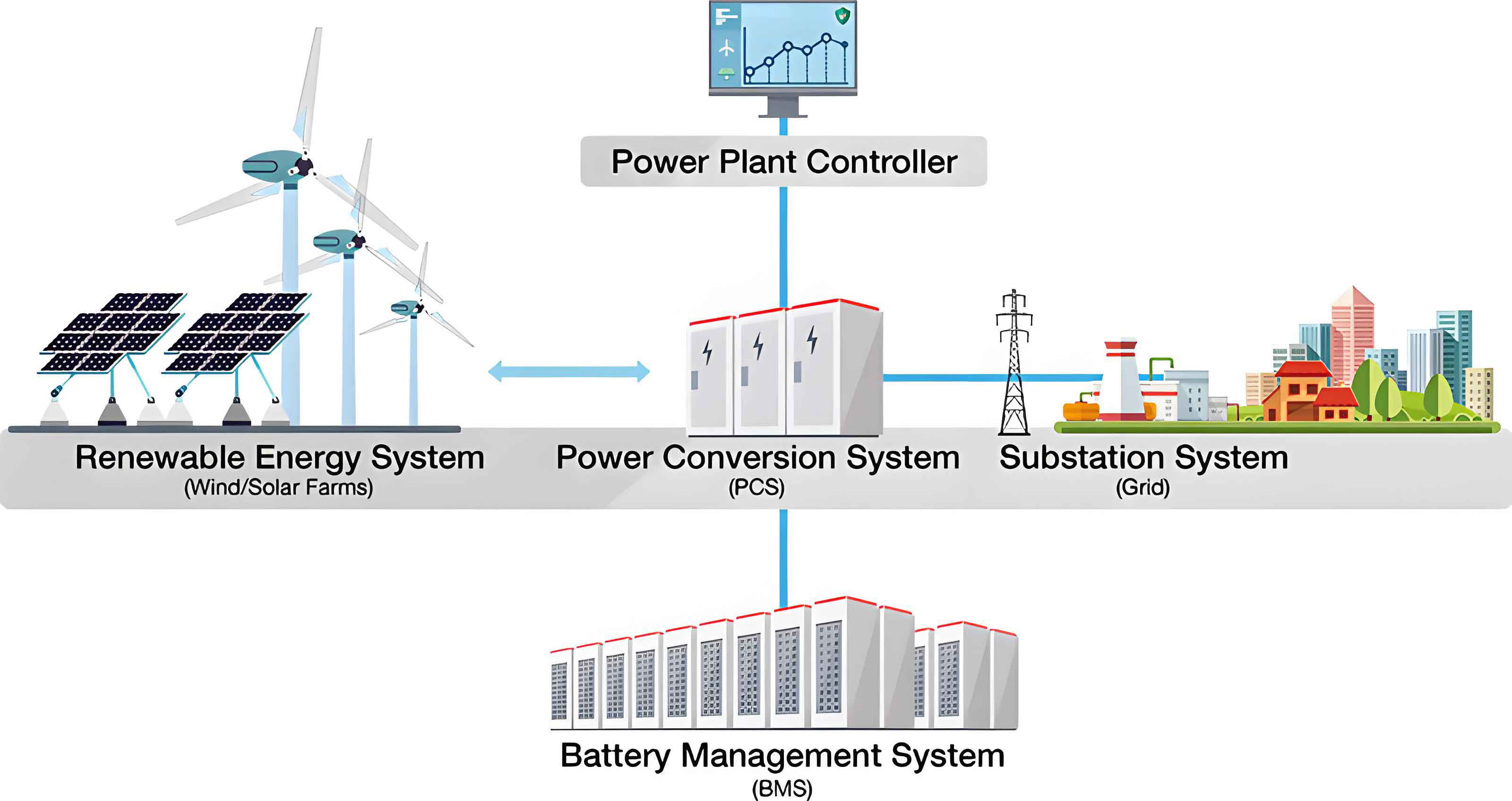
For the 5G base station energy storage system, I established a dispatchable storage model that dynamically partitions the battery capacity into reserve capacity and dispatchable capacity. The reserve capacity ensures uninterrupted base station operation during grid anomalies, while the dispatchable capacity participates in microgrid coordination. This dynamic division responds to fluctuating communication loads, enabling the energy storage system to adaptively release or restrict adjustable capacity. The capacity dynamics are described by:
$$E_i(t+1) = E_i(t)(1-\lambda_E) + \frac{P_{\rm disch}^i(t)\Delta t}{\eta_{\rm disch}} – P_{\rm ch}^i(t)\eta_{\rm ch}\Delta t$$
The minimum reserve capacity and the adjustable capacity are determined by:
$$\begin{cases}
E_i^{\rm sp}(t) = \max\{E_i^{\min}, E_i^{5G}(t)\} \\[4pt]
E_i^{\rm dpa}(t) = E_i(t) – E_i^{\rm sp}(t)
\end{cases}$$
I also developed a power consumption aggregation model based on demand response. The total power consumption of the 5G base station network comprises macro base station consumption and micro base station consumption:
$$P_{\rm total}(t) = P_m(t) + \sum_{k\in BS} P_k(t)$$
Macro base station power consumption consists of static and dynamic components related to communication traffic load. Micro base stations can operate in either active or sleep modes:
$$P_k(t) = \begin{cases}
P_{\theta}^{\rm active}, & \theta_k = 1 \\[4pt]
P_{\theta}^{\rm sleep}, & \theta_k = 0
\end{cases}$$
The bi-level optimization model for the 5G base station microgrid comprises a planning layer that minimizes the life cycle cost and a scheduling layer that minimizes daily operating costs. The planning layer objective function, incorporating construction, O&M, replacement, grid trading, and environmental protection costs, is formulated as:
$$F_{\rm LCC}^{\min} = C_n + C_{om} + C_r + C_g – R_s$$
where the net grid cost and revenue terms are:
$$C_g = \int_0^T k_{\rm buy}P_{\rm buy}(t)dt – \int_0^T k_{\rm sell}P_{\rm sell}(t)dt$$
The scheduling layer focuses on minimizing the daily operating cost of the base station cluster, constituting a critical subproblem that validates short-term dispatch efficiency of the entire energy storage system:
$$\min \ F_{\rm DC}^{5G} = C_{\rm grid}$$
Constraint conditions include power balance, output power limits for wind and photovoltaic generation, battery constraints, power exchange constraints, and load classification constraints. The system parameters adopted in the simulation include four macro base stations and three thousand micro base stations, along with four groups of 48V/100Ah lithium batteries, each having a maximum charging power of 5kW and charging efficiency of 0.95. The simulation utilized time-of-use electricity pricing and pollutant emission penalty coefficients as summarized below:
| Pollutant | Treatment Cost (CNY/kg) | PV Emission | Wind Emission | Grid Emission |
|---|---|---|---|---|
| CO₂ | 0.02 | 1.60 | 1.60 | 889.00 |
| SO₂ | 6.00 | 1.60 | 1.60 | 1.80 |
| NOₓ | 8.00 | 1.60 | 1.60 | 1.60 |
| Category | Period | Purchase Price (CNY/kWh) | Selling Price (CNY/kWh) |
|---|---|---|---|
| Peak | 08:00-12:00, 17:00-23:00 | 0.93 | 0.72 |
| Flat | 07:00-08:00, 12:00-19:00 | 0.62 | 0.53 |
| Valley | 23:00-07:00 | 0.31 | 0.28 |
I conducted a comparative simulation using PSO, GWO, BWO, and the proposed IBWO algorithms to validate the optimization capability of the improved algorithm. The convergence curves demonstrate that IBWO achieves the fastest convergence and the minimal objective value. The cost comparison results are summarized in the following table:
| Algorithm | IBWO | GWO | PSO | BWO |
|---|---|---|---|---|
| Grid Trading Cost | 22.00 | 27.60 | 28.00 | 25.00 |
| Generation Cost | 76.40 | 78.20 | 84.50 | 79.00 |
| Energy Storage Cost | 20.50 | 18.80 | 21.30 | 19.10 |
| Daily Operating Cost | 69.59 | 87.58 | 94.29 | 87.32 |
| Annual Comprehensive Cost | 43851.35 | 50328.70 | 51826.85 | 49180.80 |
Compared with PSO, GWO, and BWO, IBWO reduces the daily operating cost by 26.20%, 20.54%, and 20.30%, respectively, while the annual comprehensive cost is reduced by 12.87%, 15.39%, and 10.84%, respectively. The stacked bar chart of the capacity allocation results reveals that the energy storage system effectively achieves dynamic supply-demand matching: during periods of abundant wind power, excess energy charges the energy storage system; during peak load hours, the energy storage system discharges to compensate renewable generation insufficiency. I also evaluated the system performance under four scenarios: without energy storage dispatch and power aggregation, with only energy storage dispatch, with only power aggregation, and with the complete strategy. The results show that the scenario integrating both dispatchable energy storage and power aggregation achieves the best economic performance, with the annual comprehensive cost reduced by approximately 53.8% compared to the baseline scenario.
5. Application Case II: Hybrid Electrical-Hydrogen Storage Microgrid
To further validate the effectiveness of the proposed method in hybrid energy storage optimization, I constructed a microgrid model incorporating both battery and hydrogen energy storage systems. This configuration fully exploits the complementary characteristics of different storage technologies within the energy storage system. The system architecture integrates photovoltaic arrays, wind turbines, battery energy storage, electrolyzers, hydrogen storage tanks, fuel cells, micro gas turbines, and grid interconnection, with an Energy Management System (EMS) orchestrating the coordination of all components.
The bi-level optimization model for the hybrid energy storage microgrid consists of an outer layer aimed at minimizing the annual comprehensive cost and an inner layer responsible for minimizing grid-connected power fluctuations. The outer objective function is:
$$\min \ C_y = C_n + C_{om} + C_r + C_g + C_e$$
The initial construction cost, annual O&M cost, and replacement cost are formulated respectively as:
$$C_n = \sum_{i=1}^{n} N_i c_i^n S_i^n \beta_{\rm CRF}, \quad \beta_{\rm CRF} = \frac{k(1+k)^{Y_i}}{(1+k)^{Y_i}-1}$$
$$C_{om} = \sum_{i=1}^{n} N_i c_i^{om} S_i^n$$
$$C_r = \sum_{i=1}^{m} N_i c_i^r S_i^n \lambda_{\rm CRF}, \quad \lambda_{\rm CRF} = \frac{r}{(1+r)^{Y_i}-1}$$
The inner layer utilizes MVMD for adaptive decomposition of the wind-solar net load, establishing a multi-timescale coordinated dispatch mode between batteries and hydrogen storage. The objective function quantifies the grid-connected power fluctuation rate:
$$\Delta P(t) = \left| \frac{P_g(t) – P_g(t-1)}{P_{\rm rated}} \right| \times 100\%$$
Constraint conditions encompass power balance, wind and photovoltaic generation limits, battery charging/discharging constraints, hydrogen storage system constraints, micro gas turbine operation limitations, power exchange boundaries with the main grid, device quantity limitations, and power fluctuation limits. The power balance equation is:
$$P_{\rm wt} + P_{\rm PV} + P_{\rm BAT} + P_{\rm FC} + P_{\rm grid} + P_{\rm MT} = P_{\rm el} + P_{\rm load}$$
Based on historical data from a wind-solar demonstration base, I extracted two typical days for simulation analysis. The renewable energy curtailment rate serves as a key evaluation metric:
$$\sigma_{ab} = \frac{P_{ab}}{P_{to}} \times 100\%$$
The operational strategy of the hybrid energy storage system is driven by the net load power:
$$P_{\rm net} = P_{\rm PV} + P_{\rm wt} – P_{\rm load}$$
When \(P_{\rm net} > 0\), the surplus renewable energy is prioritized for charging the battery for high-frequency components, while the hydrogen storage system absorbs the medium and low-frequency components. When \(P_{\rm net} < 0\), the battery discharges rapidly to compensate high-frequency shortfall, followed by the hydrogen storage system handling the medium and low-frequency deficits. Should both energy storage units reach their capacity limits, the micro gas turbine is activated as the next resort, and the grid serves as the final backup. The simulation results demonstrate that the hybrid energy storage system effectively smooths the grid-connected power, with the maximum fluctuation controlled within 7.63% and the annual comprehensive cost reduced by approximately 27.5% compared to the single-layer model.
The convergence performance comparison confirms that IBWO achieves the fastest convergence rate and the lowest final objective value relative to PSO, GWO, and BWO algorithms. The capacity configuration results obtained by different algorithms are presented below:
| Algorithm | P2G | Fuel Cell | Battery Energy Storage | Hydrogen Storage | Gas Turbine | Curtailed Power |
|---|---|---|---|---|---|---|
| IBWO | 800.00 | 39.82 | 718.23 | 93.05 | 800.00 | 103.05 |
| PSO | 900.00 | 43.02 | 589.47 | 88.80 | 800.00 | 267.11 |
| BWO | 1200.00 | 43.02 | 459.72 | 108.99 | 800.00 | 276.35 |
| GWO | 1000.00 | 1118.00 | 1096.21 | 164.08 | 120.00 | 279.17 |
I also conducted multi-scenario comparative analysis by setting various configurations including single-layer optimization, bi-level optimization with only battery storage, bi-level optimization with only hydrogen storage, single-layer optimization with hybrid storage, and bi-level optimization with hybrid storage. The results clearly demonstrate that the bi-level model with hybrid electrical-hydrogen storage achieves the lowest total cost while significantly reducing the renewable energy curtailment.
| Scenario | Grid Cost | Storage Cost | Gas Cost | Environmental Cost | Oxygen Revenue | Curtailment | Total Cost |
|---|---|---|---|---|---|---|---|
| Scenario 1 | 20761.06 | 0.00 | 8052.12 | 1568.00 | 0.00 | 2015.21 | 32396.06 |
| Scenario 2 | 11863.46 | 11161.10 | 5046.05 | 1256.00 | 0.00 | 1842.10 | 31168.57 |
| Scenario 3 | 6779.12 | 9498.81 | 5023.01 | 963.33 | 4677.17 | 1785.05 | 19372.27 |
| Scenario 4 | 3873.78 | 8084.10 | 4896.20 | 963.33 | 3985.10 | 1161.51 | 14993.92 |
| Scenario 5 | 2213.59 | 6880.08 | 4482.36 | 917.46 | 4678.07 | 1054.00 | 10869.49 |
Analyzing the results across the five distinct scenarios reveals that the bi-level optimization model with integrated hybrid electrical-hydrogen storage achieves a 27.5% reduction in overall system cost compared with the single-layer hybrid storage model, while also markedly curtailing energy curtailment values and alleviating generation pressure during periods of insufficient renewable output. Through the implementation of two typical days of data, I further analyzed the system behavior under different renewable resource conditions. The capacity configuration results for the two typical days are summarized below:
| Typical Day | PV | Wind | P2G | Fuel Cell | Battery | Hydrogen Storage | Gas Turbine |
|---|---|---|---|---|---|---|---|
| Day I | 40.30 | 334.65 | 1200.00 | 32.65 | 765.30 | 297.63 | 800.00 |
| Day II | 378.91 | 320.70 | 1200.00 | 44.52 | 902.90 | 2595.12 | 800.00 |
In Typical Day II, where photovoltaic and wind power generation are considerably higher, the system increases the hydrogen storage configuration ratio substantially to accommodate surplus renewable energy. This adaptive behavior confirms the effectiveness of the model in dynamically adjusting energy storage system capacity according to varying renewable resource conditions. The MVMD optimization method adaptively determines the decomposition modal count and grid-connection modes based on signal characteristics, effectively avoiding the over-decomposition or under-decomposition problems inherent in conventional VMD methods. For Typical Day I, the optimal modal number was 1500 with one grid-connection mode, while Typical Day II required 2000 modes with two grid-connection modes, demonstrating the adaptive nature of the algorithm.
I further performed a sensitivity analysis by varying the energy storage equipment cost coefficient from 5% to 30%. The results indicate that as storage costs decrease, the hydrogen storage capacity configuration increases significantly, while the growth rate of total system cost diminishes. This trend reflects the growing economic viability of hydrogen storage as technology progresses.
| Cost Reduction | Battery Capacity | Hydrogen Capacity | Hybrid Cost | Total Cost |
|---|---|---|---|---|
| 5% | 728.67 | 107.01 | 8744.09 | 10652.10 |
| 10% | 677.90 | 102.12 | 8134.74 | 13586.52 |
| 15% | 812.30 | 125.34 | 9747.60 | 11321.05 |
| 20% | 832.61 | 188.70 | 9991.29 | 11524.05 |
| 25% | 836.77 | 190.58 | 10041.25 | 11662.33 |
| 30% | 840.95 | 223.20 | 10091.45 | 11559.71 |
6. Conclusion and Future Outlook
In this work, I systematically investigated the optimal design and operational scheduling of the energy storage system for renewable energy integration in microgrid applications. The key contributions and findings are fourfold. First, I constructed a collaborative “source-storage-load” bi-level optimization model, where the outer layer addresses long-term capacity configuration of wind turbines, photovoltaic arrays, and energy storage equipment, while the inner layer performs multi-timescale optimal operation and dispatch. The iterative interaction between these two layers achieves synergistic optimization between capacity planning and operational strategies. Second, I proposed a multi-strategy Improved Beluga Whale Optimization algorithm integrating reverse elite strategy, crisscross mechanism, and cyclone foraging strategy, which significantly enhances the global search capability and convergence precision. Ablation experiments and benchmark function tests confirmed the superiority of IBWO over PSO, GWO, and standard BWO algorithms. Third, I designed a hybrid energy storage coordination scheduling strategy based on MVMD adaptive decomposition, where battery storage manages high-frequency power fluctuations and hydrogen storage undertakes medium and low-frequency energy balancing tasks. This multi-timescale battery-hydrogen coordinated dispatch mode effectively smooths grid-connected power fluctuations. Fourth, the application of the proposed model and method in both a 5G base station microgrid and an electrical-hydrogen hybrid storage microgrid demonstrated significant improvements in system economics and operational stability. The annual comprehensive cost was reduced by approximately 53.8% in the 5G base station scenario and 27.5% in the hybrid storage scenario, with the maximum power fluctuation controlled within 7.63%.
For future research, several directions merit exploration. The scalability of the proposed approach to multi-microgrid energy sharing and collaborative dispatch deserves further investigation. The integration of system resilience, user satisfaction, and market mechanisms into the optimization framework presents an interesting multi-objective extension. Additionally, incorporating equipment degradation, battery life attenuation, and time-varying cost factors into the capacity planning and scheduling models would enhance the practical applicability of the proposed method. As the energy storage system continues to evolve with advancing technology and declining costs, the proposed framework provides a robust foundation for the development of low-carbon, efficient, and reliable microgrid systems.