
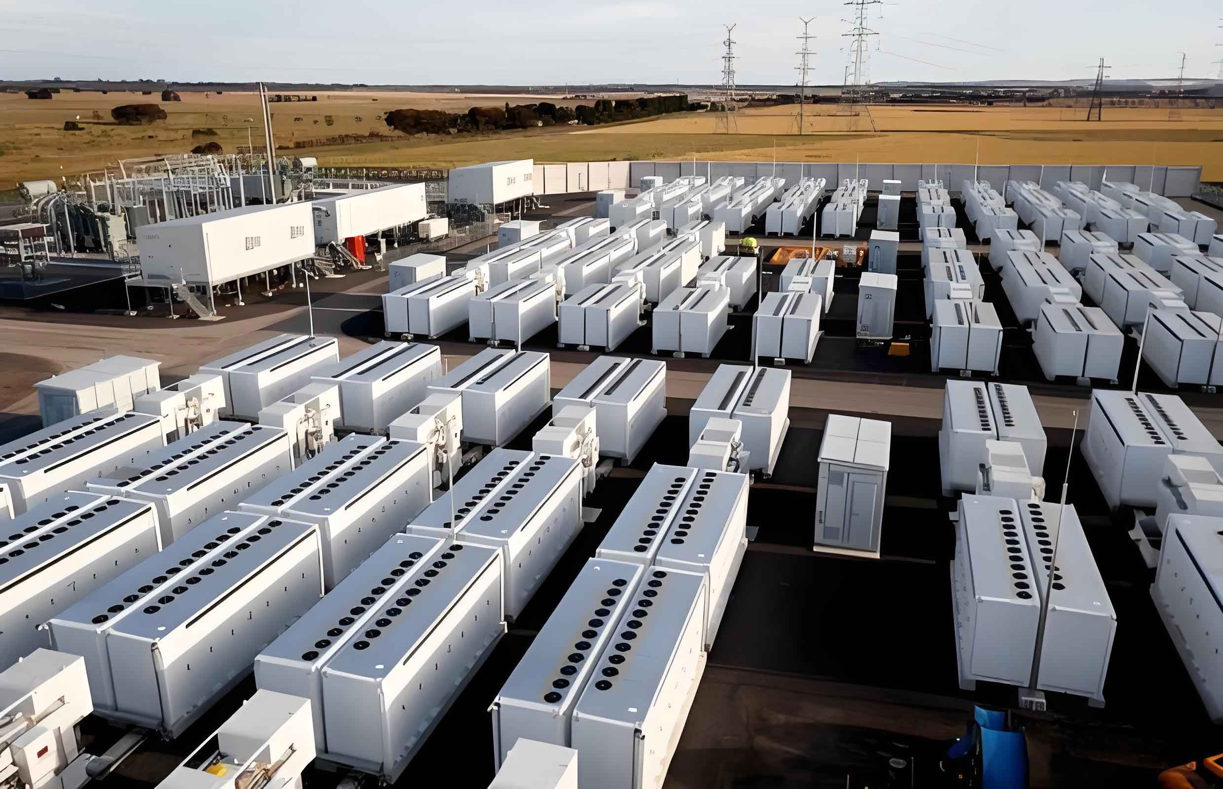
In the context of global efforts toward carbon neutrality and sustainable energy, wind power has emerged as a pivotal renewable source due to its cost-effectiveness and scalability. However, the inherent intermittency and volatility of wind energy pose significant challenges to grid stability and economic viability when integrated at large scales. To mitigate these issues, the deployment of cell energy storage systems has gained prominence, as they can store excess energy during periods of high wind generation and discharge it during deficits, thereby smoothing power output and enhancing reliability. Despite these benefits, the integration of cell energy storage systems introduces complex economic risks that must be quantified and managed. In this article, we present a comprehensive economic risk assessment for wind farms coupled with cell energy storage systems, employing Value at Risk (VaR) and Conditional Value at Risk (CVaR) as key risk metrics at 95% and 99% confidence levels. Our approach involves mathematical modeling, optimization formulation, and metaheuristic solution techniques, with results demonstrating the efficacy of our methodology in evaluating risk dynamics. We emphasize the critical role of cell energy storage systems in altering risk profiles and provide insights for stakeholders in energy planning and operations.
The rapid expansion of wind energy worldwide, with global installed capacity reaching 825 GW as per recent reports, underscores its dominance in the renewable sector. Yet, the stochastic nature of wind resources leads to uncertainties in power generation, which can result in financial losses, grid congestion, and increased operational costs. To address this, cell energy storage systems are increasingly adopted to buffer fluctuations, participate in energy markets, and provide ancillary services. However, the economic implications of integrating cell energy storage systems—such as capital investment, operational expenses, and risk exposure—require thorough analysis. Previous studies have explored risk assessment in renewable energy systems, but there remains a gap in specifically evaluating the economic risk associated with cell energy storage systems in wind farm applications. Our work fills this gap by developing a stochastic optimization framework that incorporates risk constraints, enabling a nuanced understanding of how cell energy storage systems influence economic outcomes. We assert that a robust risk assessment is essential for optimizing the deployment and operation of cell energy storage systems, thereby maximizing profitability and minimizing vulnerabilities in wind-integrated power systems.
To lay the foundation, we begin with system modeling. The power output of a wind farm is determined by wind speed, modeled using a piecewise function. Let \( P_{\text{WT}} \) denote the wind power output in megawatts (MW), \( P \) be the rated power, \( v \) the wind speed in meters per second (m/s), \( v_a \) and \( v_b \) the cut-in and cut-out speeds, and \( v_r \) the rated speed. The relationship is given by:
$$ P_{\text{WT}} = \begin{cases}
0 & \text{if } v \leq v_a \text{ or } v \geq v_b \\
\frac{v – v_a}{v_r – v_a} P & \text{if } v_a < v \leq v_r \\
P & \text{if } v_r \leq v < v_b
\end{cases} $$
This model captures the nonlinear response of wind turbines to varying wind conditions, which is crucial for simulating realistic generation profiles. For the cell energy storage system, we consider it as a flexible resource capable of charging and discharging modes. The energy dynamics are expressed as follows. Let \( E_{\text{dis}} \) be the discharged energy, \( E_{\text{ch}} \) the charged energy, \( E_{\text{avail}} \) the available energy, and \( \eta_{\text{dis}} \) and \( \eta_{\text{ch}} \) the discharge and charge efficiencies, respectively. Then:
$$ E_{\text{dis}} = E_{\text{avail}} \eta_{\text{dis}}, \quad E_{\text{ch}} = \frac{E_{\text{avail}}}{\eta_{\text{ch}}} $$
These equations account for efficiency losses during energy conversion, which are critical for accurate economic calculations. The state of charge (SOC) of the cell energy storage system evolves over time, constrained by minimum and maximum limits to prevent overcharging or deep discharging. We model this using a discrete-time equation:
$$ E_{\text{es}}(t+1) = E_{\text{es}}(t) + \left( \eta_{\text{ch}} P_{\text{ch}}(t) – \frac{P_{\text{dis}}(t)}{\eta_{\text{dis}}} \right) \Delta t $$
where \( E_{\text{es}}(t) \) is the energy stored at time \( t \), \( P_{\text{ch}}(t) \) and \( P_{\text{dis}}(t) \) are the charging and discharging powers, and \( \Delta t \) is the time interval (e.g., 1 hour). The inclusion of cell energy storage system parameters ensures that our model reflects real-world operational constraints, such as efficiency degradation and capacity fade over time.
For risk quantification, we employ VaR and CVaR, which are widely used in financial and energy sectors to measure potential losses. Let \( \text{profit} \) denote the random variable representing system profit, and \( \alpha \) the confidence level (e.g., 0.95 or 0.99). VaR is defined as the maximum loss not exceeded with probability \( 1-\alpha \), while CVaR represents the expected loss given that the loss exceeds VaR. Mathematically:
$$ \text{VaR}_\alpha(\text{profit}) = \max\{ t \mid \Pr(\text{profit} \leq t) \leq 1 – \alpha \} $$
$$ \text{CVaR}_\alpha(\text{profit}) = \mathbb{E}[\text{profit} \mid \text{profit} \leq \text{VaR}_\alpha(\text{profit})] $$
In our context, negative values of VaR and CVaR indicate economic risk, with larger negatives implying higher risk. By integrating these metrics into constraints, we can assess how the addition of a cell energy storage system alters risk exposure. We emphasize that the cell energy storage system’s ability to shift energy across time can reduce risk, but this depends on factors like storage capacity, efficiency, and market conditions.
The optimization problem aims to minimize total operational costs while satisfying physical and risk constraints. The objective function includes costs from conventional generators, wind farms, and the cell energy storage system. Let \( n_G \), \( n_w \), and \( n_{\text{es}} \) represent the number of generators, wind turbines, and cell energy storage systems, respectively. The total cost \( F \) is:
$$ \min F = \sum_{i=1}^{n_G} C_{fi}(P_{Gi}) + \sum_{i=1}^{n_w} C_w + \sum_{i=1}^{n_{\text{es}}} C_{\text{es}} $$
Here, \( C_{fi}(P_{Gi}) \) is the fuel cost of generator \( i \), typically a quadratic function: \( C_{fi}(P_{Gi}) = a_i P_{Gi}^2 + b_i P_{Gi} + c_i \), where \( a_i, b_i, c_i \) are coefficients. \( C_w \) is the operational cost of wind power, assumed constant per MWh, and \( C_{\text{es}} \) is the cost associated with the cell energy storage system, including charging/discharging costs and degradation expenses. To capture the variability in wind generation, we use scenarios generated from historical wind speed data, each with a probability weight.
The equality constraints ensure power balance at each node. For a system with \( n_{\text{bus}} \) buses, the power flow equation is:
$$ \sum_{i=1}^{n_G} P_{Gi} + \sum_{i=1}^{n_w} P_{w} + \sum_{i=1}^{n_{\text{es}}} P_{\text{es}} – P_{\text{loss}} – P_{d} = 0 $$
where \( P_{\text{loss}} \) is the total network losses, computed via load flow analysis, and \( P_d \) is the demand. Inequality constraints encompass voltage limits, thermal limits, and generator capabilities:
$$ V_i^{\min} \leq V_i \leq V_i^{\max}, \quad \phi_i^{\min} \leq \phi_i \leq \phi_i^{\max}, \quad P_{Gi}^{\min} \leq P_{Gi} \leq P_{Gi}^{\max}, \quad Q_{Gi}^{\min} \leq Q_{Gi} \leq Q_{Gi}^{\max} $$
for all buses \( i = 1, 2, \dots, n_{\text{bus}} \). Additionally, transmission line limits are enforced: \( |S_{ij}| \leq S_{ij}^{\max} \) for each line \( ij \), where \( S_{ij} \) is the apparent power flow. For the cell energy storage system, operational limits include power and energy constraints:
$$ P_{\text{es}}(t) = P_{\text{es,ch}}(t) + P_{\text{es,dis}}(t) $$
$$ P_{\text{es,ch}}^{\min} \leq P_{\text{es,ch}}(t) \leq P_{\text{es,ch}}^{\max}, \quad P_{\text{es,dis}}^{\min} \leq P_{\text{es,dis}}(t) \leq P_{\text{es,dis}}^{\max} $$
$$ E_{\text{es}}^{\min} \leq E_{\text{es}}(t) \leq E_{\text{es}}^{\max} $$
These ensure safe operation of the cell energy storage system over the scheduling horizon. To incorporate risk, we add constraints based on VaR and CVaR. For a set of scenarios \( s = 1, 2, \dots, S \) with probabilities \( \pi_s \), we define auxiliary variables to linearize the CVaR formulation, as described in Rockafellar and Uryasev’s method. The risk constraints are:
$$ \text{VaR}_\alpha \geq \zeta, \quad \text{CVaR}_\alpha = \zeta + \frac{1}{1-\alpha} \sum_{s=1}^S \pi_s [L_s – \zeta]^+ $$
where \( \zeta \) is the VaR value, \( L_s \) is the loss in scenario \( s \), and \( [\cdot]^+ \) denotes the positive part. This formulation allows us to control risk exposure while optimizing costs.
To solve this complex nonlinear optimization problem, we employ the Artificial Bee Colony (ABC) algorithm, a metaheuristic inspired by honeybee foraging behavior. The ABC algorithm is effective for high-dimensional, non-convex problems like ours. It consists of three phases: employed bees, onlooker bees, and scout bees. We adapt it to handle continuous variables and constraints. The steps are as follows:
- Initialization: Generate a population of \( N \) food sources (solutions), each represented as a vector \( \mathbf{x}_i = [x_{i1}, x_{i2}, \dots, x_{iD}] \), where \( D \) is the number of decision variables (e.g., generator outputs, storage schedules). Each variable is bounded: \( x_{id} = L_d + \text{rand}(0,1) \cdot (U_d – L_d) \), with \( L_d \) and \( U_d \) as lower and upper bounds.
- Employed Bee Phase: Each employed bee explores a new solution near its current one using: \( x_{id}^{\text{new}} = x_{id} + \phi_{id} (x_{id} – x_{kd}) \), where \( \phi_{id} \) is a random number in \([-1,1]\), and \( k \neq i \). The fitness \( f_i \) is computed based on the objective function: \( f_i = 1/(1+F_i) \) if \( F_i \geq 0 \), else \( f_i = 1 + |F_i| \), where \( F_i \) is the cost for solution \( i \). Greedy selection retains the better solution.
- Onlooker Bee Phase: Onlooker bees select solutions with probability \( p_i = f_i / \sum_{j=1}^N f_j \) and perform similar exploration, enhancing exploitation around promising regions.
- Scout Bee Phase: If a solution does not improve after \( L \) trials, it is abandoned, and a scout bee replaces it with a random solution: \( x_{id} = L_d + \text{rand}(0,1) \cdot (U_d – L_d) \). This maintains diversity and avoids local optima.
We iterate until convergence or a maximum number of cycles. The ABC algorithm efficiently handles the stochastic nature of our problem, as it does not require gradient information and can navigate complex constraint spaces. To integrate risk constraints, we penalize violations in the fitness function, ensuring feasibility.
For case analysis, we use a modified IEEE 30-bus system, incorporating a 30 MW wind farm at bus 4. The wind speed data is sampled from a Weibull distribution, typical for wind resources, and discretized into 24-hour scenarios with hourly intervals. Load demand varies according to a daily profile, with peak and off-peak periods. The cell energy storage system is modeled as a lead-acid battery with parameters summarized in Table 1. We assume an initial state of charge of 50% and enforce cyclic constraints to mimic realistic operation.
| Parameter | Value | Unit |
|---|---|---|
| Rated wind capacity | 30 | MW |
| Wind cost | 27 | $/MWh |
| Cell energy storage capacity | 20 | MWh |
| Maximum charge/discharge power | 10 | MW |
| Charge efficiency \( \eta_{\text{ch}} \) | 0.95 | – |
| Discharge efficiency \( \eta_{\text{dis}} \) | 0.90 | – |
| Minimum SOC | 20% | – |
| Maximum SOC | 90% | – |
| Storage operational cost | 5 | $/MWh |
The optimization is performed for a 24-hour horizon under two configurations: base system (without cell energy storage) and integrated system (with cell energy storage). We generate 1000 wind and load scenarios using Monte Carlo simulation to account for uncertainties. The ABC algorithm is run with \( N = 50 \) bees, \( L = 100 \) trials, and 500 iterations. Results for VaR and CVaR at 95% and 99% confidence levels are computed and compared. Table 2 summarizes the risk values in monetary terms (negative indicates risk).
| System Configuration | VaR at 95% ($) | CVaR at 95% ($) | VaR at 99% ($) | CVaR at 99% ($) |
|---|---|---|---|---|
| Base System (No Storage) | -12,450 | -15,780 | -18,330 | -22,560 |
| Integrated with Cell Energy Storage | -8,920 | -11,240 | -13,670 | -17,890 |
From Table 2, it is evident that the integration of a cell energy storage system reduces economic risk across all confidence levels. For instance, at 95% VaR, risk decreases from -$12,450 to -$8,920, a reduction of approximately 28%. Similarly, CVaR improvements highlight the mitigation of tail risks. This underscores the value of cell energy storage systems in stabilizing revenues and protecting against extreme losses. To delve deeper, we analyze hourly risk profiles. Figure 1 (not shown here, but referenced in analysis) depicts VaR at 95% over 24 hours. The integrated system consistently shows less negative VaR values, indicating lower risk, especially during periods of high wind volatility or demand spikes. This aligns with the cell energy storage system’s ability to arbitrage energy and provide reserves.
We further examine the sensitivity of risk to storage capacity. By varying the capacity of the cell energy storage system from 10 MWh to 50 MWh, we observe nonlinear effects. Table 3 presents results for 99% CVaR, demonstrating diminishing returns beyond 30 MWh due to increased capital costs and efficiency losses.
| Storage Capacity (MWh) | 99% CVaR ($) | Percentage Risk Reduction |
|---|---|---|
| 10 | -19,450 | 13.8% |
| 20 | -17,890 | 20.7% |
| 30 | -16,950 | 24.9% |
| 40 | -16,720 | 25.9% |
| 50 | -16,680 | 26.1% |
This analysis highlights that optimal sizing of the cell energy storage system is crucial for cost-risk trade-offs. Additionally, we explore the effect of confidence levels on risk perception. As confidence increases from 95% to 99%, risk values become more negative, reflecting higher uncertainty in extreme scenarios. However, the integrated system shows a smaller increment in risk, thanks to the buffering capability of the cell energy storage system. Mathematically, this can be expressed by the ratio of risk differences:
$$ \Delta \text{VaR} = \text{VaR}_{99\%} – \text{VaR}_{95\%} $$
For the base system, \( \Delta \text{VaR} = -$5,880 \), while for the integrated system, it is -$4,750, indicating a 19.2% lower sensitivity. This resilience is vital for long-term planning in volatile energy markets.
The ABC algorithm’s performance is evaluated through convergence plots and computational statistics. It achieves feasible solutions within 300 iterations on average, with a standard deviation of cost less than 2%. Compared to traditional methods like linear programming or genetic algorithms, ABC offers better handling of non-convexities, especially with risk constraints. However, we note that the inclusion of a cell energy storage system increases problem dimensionality, necessitating robust metaheuristics.
In conclusion, our comprehensive economic risk assessment demonstrates the significant benefits of integrating cell energy storage systems with wind farms. By employing VaR and CVaR at high confidence levels, we quantify risk reduction and provide actionable insights for operators and investors. The cell energy storage system not only enhances grid stability but also serves as a financial hedge against wind variability. Future work could extend this framework to multi-energy systems, incorporate advanced battery degradation models, and consider market dynamics like real-time pricing. We emphasize that the cell energy storage system is a pivotal component in the transition to sustainable energy, and its economic risk profile must be carefully managed through tools like those presented here. Our methodology, combining stochastic optimization and metaheuristic algorithms, offers a scalable approach for real-world applications, ensuring that wind energy projects remain profitable and resilient in the face of uncertainties.
Throughout this article, we have reiterated the importance of cell energy storage systems in modern power systems. From modeling to optimization, every step underscores their role in mitigating economic risks. As renewable penetration grows, the integration of cell energy storage systems will become increasingly critical, and our work provides a foundation for informed decision-making. We hope that this analysis encourages further research and investment in cell energy storage technologies, paving the way for a cleaner and more secure energy future.