
In recent years, the rapid growth of global energy demand has accelerated the transition from traditional fossil fuels to renewable energy sources. Among these, solar photovoltaic power generation has become one of the most promising alternatives due to its low cost, wide availability, and low carbon emissions. Consequently, the photovoltaic industry has expanded dramatically worldwide. To optimize power system planning and facilitate the stable integration of solar energy into the grid, accurate information about the installed capacity and geographic distribution of solar panels is essential. Remote sensing imagery, which covers large areas and provides consistent observations, has become a powerful tool for monitoring ground objects. Meanwhile, deep learning techniques have demonstrated outstanding performance in various remote sensing tasks including semantic segmentation. However, the automatic extraction of solar panels from remote sensing images remains challenging due to limited data samples, complex backgrounds, imbalanced object categories, and the low spatial resolution of many satellite images. In this thesis, I focus on addressing these challenges by designing deep learning models that can accurately segment solar panels from high-resolution and low-resolution remote sensing images. I first construct a distributed solar panel dataset to enhance model generalization. Then, I propose two improved segmentation algorithms: one based on attention mechanisms and global convolution, and another based on multi-level feature fusion with self-convolution. Extensive experiments demonstrate that the proposed methods achieve high precision and robust performance on multiple public datasets.
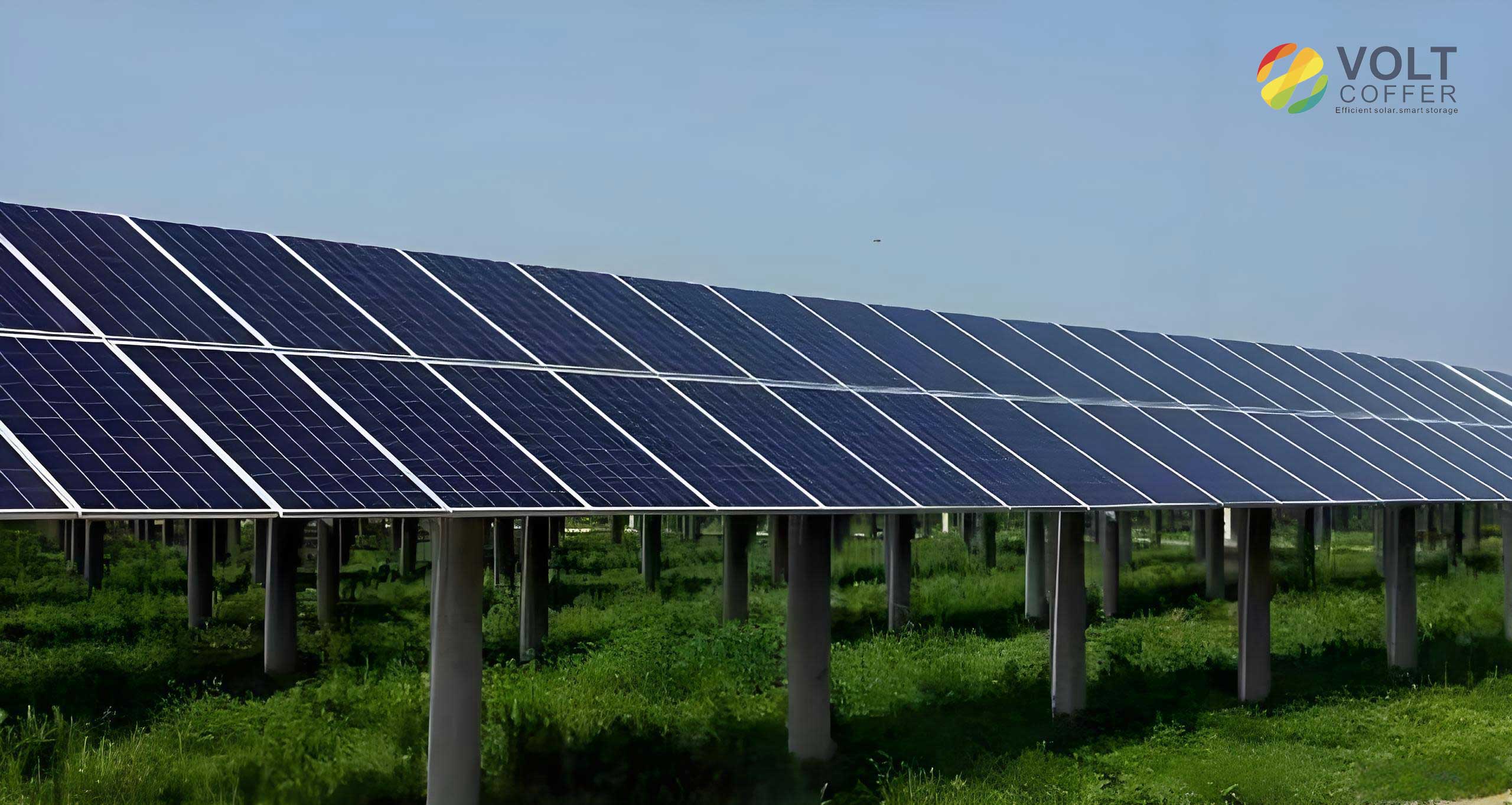
Background and Problem Analysis
Solar panels can be generally classified into two categories: centralized photovoltaic (PV) plants and distributed photovoltaic systems. Centralized plants are usually installed in remote areas such as deserts and Gobi regions, where the background is relatively simple. In contrast, distributed solar panels are often mounted on rooftops, agricultural greenhouses, or water surfaces, leading to complex backgrounds and high variability in appearance. The spatial resolution of remote sensing imagery significantly affects the accuracy of solar panel extraction. When the resolution is lower than 0.6 meters, the recognition accuracy drops sharply. High-resolution images with a spatial resolution of 0.1 to 0.3 meters can provide sufficient detail for precise extraction. Nevertheless, even with high-resolution data, several obstacles remain: (1) solar panels often have colors similar to rooftops or surrounding terrain; (2) the proportion of solar panel pixels in the entire image can be extremely imbalanced; (3) adjacent panels may appear merged due to low resolution or shadow effects; and (4) some objects like agricultural greenhouses or reflective surfaces can mimic the spectral signature of solar panels. Traditional image processing methods rely on manually designed features such as edges and geometric properties, which are not robust enough for diverse scenarios. Machine learning methods using hand-crafted features require extensive preprocessing and still struggle with complex backgrounds. Deep learning, especially fully convolutional networks, offers an end-to-end solution that learns hierarchical features directly from data. However, generic segmentation architectures such as U-Net, SegNet, or DeepLabv3+ often produce coarse boundaries or miss small distributed arrays. Therefore, I propose tailored improvements to address these issues.
Dataset Construction and Augmentation
To train and evaluate the proposed models, I utilize three public datasets obtained from Zenodo, which contain solar panel images collected by Gaofen-2, Beijing-2, and unmanned aerial vehicles in Jiangsu Province, China. These datasets are denoted as PV01, PV03, and PV08, with spatial resolutions of 0.1 m, 0.3 m, and 0.8 m, respectively. PV01 contains rooftop solar panels on concrete, steel tile, and brick backgrounds; PV03 includes rooftop, shrub, grassland, farmland, saline-alkali, and water-surface solar panels; PV08 contains rooftop and ground-mounted solar panels. The image sizes are 256×256 for PV01 and 1024×1024 for PV03 and PV08. Table 1 summarizes the composition of these datasets.
| Dataset | Solar panel type | Spatial resolution (m) | Image size | Number of images |
|---|---|---|---|---|
| PV01 | Rooftop (concrete, steel, brick) | 0.1 | 256×256 | 645 |
| PV03 | Rooftop, shrub, grass, farmland, saline, water | 0.3 | 1024×1024 | 2308 |
| PV08 | Rooftop, ground | 0.8 | 1024×1024 | 763 |
In addition to these public datasets, I construct a distributed solar panel dataset from two foreign sources: the USGS aerial orthoimagery dataset and the MAXAR distributed PV dataset. The original images are large (e.g., 6000×4000 or 4000×4000) and contain geographic coordinates. I first filter out images without solar panels, then crop the images into 512×512 patches using a sliding window with stride 512. The panels are labeled using the LabelMe annotation tool, and the resulting JSON files are converted into binary masks. After removing most empty patches, I obtain 1118 images containing distributed solar panels. Some examples are shown in Figure 1 (not referenced here due to formatting constraints). To increase data diversity and reduce overfitting, I apply a series of data augmentation techniques, including rotations of 90°, 180°, and 270°, horizontal and vertical flipping, random cropping, noise addition, color darkening, and gamma correction. These operations help the model become more robust to brightness variations, different viewing angles, and scale changes.
Method 1: Attention and Global Convolution for Solar Panel Segmentation
Overall Architecture
The first model improves the DeepLabv3+ network by integrating multiple enhancements. The backbone is ResNet-101, which extracts hierarchical features from the input image. I insert a dual attention module (DA) after the second residual block to capture spatial and channel dependencies. In the skip connections, I place a channel attention module (CAM) before a parallel combination of global convolution modules (GCM) and a fused boundary refinement (BR) module. The decoder progressively upsamples the feature maps while fusing multi-level features. An Atrous Spatial Pyramid Pooling (ASPP) module is applied after the second upsampling stage to aggregate multi-scale contextual information. Finally, a channel fusion module (CFM) is designed to recover lost channel information during upsampling. The overall structure is illustrated in the previous section.
Dual Attention Module
The dual attention module consists of a spatial self-attention branch and a channel self-attention branch. For the spatial branch, given an input feature map \(A \in \mathbb{R}^{C \times H \times W}\), I generate three feature maps \(B\), \(C\), and \(D\) using 1×1 convolutions, where \(B\) and \(C\) are reshaped to \(C \times N\) with \(N=H \times W\). The spatial attention matrix \(S\) is computed as:
$$
S_{ji} = \frac{\exp(B_i \cdot C_j)}{\sum_{i=1}^{N} \exp(B_i \cdot C_j)}
$$
where \(S_{ji}\) represents the relationship between spatial position \(i\) and position \(j\). The output feature map \(E_j\) is obtained by aggregating all positions weighted by the attention matrix and adding the original features:
$$
E_j = \sum_{i=1}^{N} S_{ji} D_i + A_j
$$
Similarly, the channel attention branch computes a channel attention matrix \(X_{ji}\) by performing matrix multiplication between \(A\) and its transpose:
$$
X_{ji} = \frac{\exp(A_i \cdot A_j)}{\sum_{i=1}^{C} \exp(A_i \cdot A_j)}
$$
The channel-refined feature map is then computed as:
$$
E_j = \sum_{i=1}^{C} X_{ji} A_i + A_j
$$
By placing the dual attention module after the second residual block, the model can focus on important spatial regions and meaningful channels while suppressing irrelevant background information. The visualization of attention weights confirms that the added module highlights the solar panel regions more clearly compared to the baseline.
Parallel Global Convolution and Fused Boundary Refinement
The global convolution module (GCM) from the Global Convolutional Network uses large separable kernels to capture global context. A \(k \times k\) convolution is decomposed into \(k \times 1\) and \(1 \times k\) convolutions, which significantly reduces parameters while maintaining a large receptive field. The GCM is constructed as a symmetric parallel structure, as shown in the original formulation. I set the kernel size \(k=9\), and the output channel number is half of the input channels to preserve channel information. In the skip connections, I combine different GCMs with a fused boundary refinement (BR) module in parallel. The BR module is a residual block with a 3×3 convolution followed by ReLU activation. I investigated several fusion strategies for the BR module, including serial and dense connections. Table 2 reports the accuracy of different BR fusion forms on the PV01 dataset.
| Module | PA | IoU |
|---|---|---|
| BR (single) | 97.30 | 87.11 |
| BR_S2 | 97.58 | 88.93 |
| BR_S3 | 97.60 | 88.91 |
| BR_S4 | 97.60 | 88.87 |
| BR_Dense2 | 96.59 | 85.40 |
| BR_Dense3 | 95.84 | 84.69 |
| BR_Dense4 | 95.37 | 84.11 |
It can be observed that the serial combination of two BR blocks (BR_S2) provides the best trade-off between accuracy and parameter overhead. Therefore, I use BR_S2 as the fused boundary refinement module. The parallel connection of GCM and BR enables the model to capture both coarse global context and fine local details simultaneously.
Channel Fusion Module
During the upsampling process, the number of channels is drastically reduced, which may cause the loss of important semantic information. To mitigate this issue, I propose a channel fusion module that concatenates the final upsampled feature map with the original input image along the channel dimension. This operation allows the decoder to access raw pixel-level information and recover some of the lost channel details. The fused feature is then passed through a fused BR module and a 1×1 convolution to produce the final segmentation map.
Ablation Study for Method 1
To validate the contribution of each component, I conduct ablation experiments on the PV01, PV03, and PV08 datasets. The baseline is DeepLabv3 with a ResNet-101 backbone. I incrementally add the traditional GCM and fused BR (denoted as TGB), the dual attention module (DA), the parallel GCM and fused BR (PGB), the channel attention module (CAM), and the channel fusion module (CFM). Table 3 shows the results on PV01.
| Method | PA | IoU | MIoU |
|---|---|---|---|
| DeepLabv3 | 95.07 | 83.19 | 81.16 |
| +TGB | 96.12 | 84.67 | 83.97 |
| +TGB+DA | 97.10 | 85.77 | 84.21 |
| +PGB+DA | 97.58 | 86.93 | 84.88 |
| +PGB+DA+CAM | 97.80 | 87.00 | 85.71 |
| +PGB+DA+CAM+CFM | 97.96 | 87.02 | 86.74 |
Similar improvements are observed on PV03 and PV08. For instance, on PV03, the IoU increases from 91.02% to 92.98% after all modules are added. On PV08, the IoU increases from 87.48% to 88.43%. The visual comparisons show that the proposed method effectively reduces missed detections, suppresses false positives, and produces smoother boundaries, especially for clustered solar panels.
Method 2: Multi-Level Feature Fusion with Self-Convolution
Overall Architecture
The second model aims to improve the segmentation of distributed solar panels from low-resolution remote sensing images. The network follows an encoder-decoder structure with ResNet-50 as the backbone. At each skip connection, I place a U-shaped fine-grained information capture module (U-FICM) and a resolution amplification perceptual information module (RAPIM) in parallel. The decoder fuses neighboring level features to recover fine details. A deep supervision method (DSM) is applied to all decoder outputs. The overall architecture is shown in the corresponding section.
U-shaped Fine-grained Information Capture Module
The U-FICM is inspired by the U-Net architecture and is designed to extract fine-grained features while filtering out redundant information. The module takes an input feature map \(F \in \mathbb{R}^{C \times H \times W}\) and performs a number of downsampling operations determined by a depth parameter \(Deep\). Each downsampling step consists of a max-pooling layer, a convolution layer, a batch normalization layer, and a ReLU activation. The convolution operation uses the proposed self-convolution (SConv) kernel, which is described next. After reaching the desired depth, the feature map is upsampled back to the original resolution and added to the input feature map. The algorithm can be summarized as follows:
|
Input: feature map \(F \in \mathbb{R}^{C \times H \times W}\), depth \(Deep\) Output: refined feature map \(O\) Initialize max-pooling layer with stride 2; self-convolution layer SConv; batch-norm; ReLU. while \(Deep \neq 0\): \(F_1 = \text{MaxPool}(F)\) \(F_2 = \text{SConv}(F_1)\) \(F_3 = \text{BatchNorm}(F_2)\) \(F_4 = \text{ReLU}(F_3)\) \(F = F_4\) \(Deep = Deep – 1\) end while \(F_5 = \text{Upsampling}(F_4)\) to original size \(O = F + F_5\) |
Through several downsampling operations, the module removes noise and retains important contextual details. Experiments reveal that placing U-FICM in the shallow layers (after the first two residual blocks) yields the best performance, because the feature map resolution is still large enough to benefit from additional downsampling without losing too much semantic information.
Self-Convolution (SConv)
Traditional convolution kernels are initialized randomly and optimized through backpropagation. I propose a self-convolution method that generates convolution kernels directly from the feature map itself. The process begins by unfolding the input feature map into a two-dimensional matrix \(M_1 \in \mathbb{R}^{(C \cdot K \cdot K) \times L}\), where \(L\) is the number of sliding windows. This matrix is then split into \(N\) groups, where \(N\) is the desired number of output channels. Adaptive average pooling and adaptive max pooling are applied to each group to capture both the average and the most prominent features. The pooled matrices are concatenated along the \(N\) dimension, and a fully connected layer is used to learn the relationships between features. The resulting weights are reshaped into \(N\) convolution kernels of size \(K \times K\). Finally, these kernels are convolved with the original feature map to produce the output. The self-convolution algorithm is detailed as follows:
|
Input: feature map \(X \in \mathbb{R}^{C \times H \times W}\) Output: feature map \(Y\) \(M_1 = \text{unfold}(X, K, \text{stride})\) Split \(M_1\) into \(N\) groups along the spatial dimension. \(\text{avg} = \text{AdaptiveAvgPool1d}(M_1)\) \(\text{max} = \text{AdaptiveMaxPool1d}(M_1)\) \(M_{\text{cat}} = \text{Concat}(\text{avg}, \text{max})\) \(M_{\text{lin}} = \text{Linear}(M_{\text{cat}})\) \(W_{\text{kernel}} = \text{Reshape}(M_{\text{lin}})\) \(Y = \text{Conv2d}(X, W_{\text{kernel}})\) |
By generating kernels based on the input’s own statistics, the convolution becomes more adaptive and generalizes better across different data distributions. The use of both average and max pooling provides complementary information: average pooling captures global tendencies, while max pooling preserves salient local details.
Resolution Amplification Perceptual Information Module
To handle low-resolution remote sensing images, the RAPIM module increases the spatial resolution of the feature map before extracting fine details. Specifically, the input feature map is first upsampled by a factor of 2 using bilinear interpolation. Then, a 3×3 convolution followed by ReLU is applied to extract local features, and a 1×1 convolution restores the original resolution. This branch produces a feature map \(A\). Simultaneously, the original feature map is passed through a GCM and a global convolution branch, yielding feature maps \(B\) and \(C\), respectively. The output is the element-wise sum of \(A\), \(B\), and \(C\):
$$
O_{\text{RAPIM}} = A + B + C
$$
The GCM uses a large kernel size \(K\), typically 9, to capture global context, while the conventional convolution in the upsampled branch captures fine spatial details. This combination compensates for the loss of boundary information in low-resolution images.
Deep Supervision Method
To improve convergence and accuracy, I apply deep supervision to all four decoder stages. Each decoder output feature map is processed by a 3×3 convolution, then upsampled to the full resolution. These side outputs are averaged to form a single prediction map used in the loss computation:
$$
\hat{y} = \frac{1}{4} \sum_{i=1}^{4} \hat{y}_i
$$
The loss is the binary cross-entropy between the averaged prediction and the ground truth mask:
$$
L_{\text{BCE}} = – \left[ y \log(\hat{y}) + (1-y) \log(1-\hat{y}) \right]
$$
This simple deep supervision mechanism accelerates backpropagation and enables each decoder branch to learn meaningful representations.
Ablation Study for Method 2
I first investigate the optimal placement and depth of U-FICM. Table 4 reports the results of using different module combinations among the four residual blocks (R1 to R4). The values in the table indicate the depth \(Deep\) for each inserted U-FICM. A depth of 0 means no module is added.
| Dataset | Location (depth) | PA | CPA | IoU | Recall | F1 |
|---|---|---|---|---|---|---|
| PV01 | R1,R2,R3,R4 (0,0,0,0) | 97.60 | 93.69 | 87.64 | 92.77 | 93.23 |
| R1,R2,R3,R4 (5,3,2,1) | 97.51 | 91.76 | 86.33 | 91.10 | 91.43 | |
| R1,R2,R3 (5,4,3) | 97.42 | 93.57 | 88.35 | 92.71 | 93.14 | |
| R1,R2 (3,2) | 97.57 | 93.39 | 88.43 | 92.01 | 92.69 | |
| PV03 | R1,R2,R3,R4 (0,0,0,0) | 98.45 | 97.61 | 89.90 | 91.94 | 94.69 |
| R1,R2,R3,R4 (5,3,2,1) | 98.20 | 97.69 | 88.54 | 92.14 | 95.08 | |
| R1,R2,R3 (5,4,3) | 98.31 | 97.85 | 88.34 | 91.48 | 94.56 | |
| R1,R2 (3,2) | 98.19 | 97.80 | 88.91 | 92.08 | 94.85 | |
| PV08 | R1,R2,R3,R4 (0,0,0,0) | 98.36 | 91.42 | 87.67 | 89.79 | 90.08 |
| R1,R2,R3,R4 (5,3,2,1) | 98.31 | 91.79 | 88.01 | 88.86 | 90.30 | |
| R1,R2,R3 (5,4,3) | 98.50 | 91.30 | 89.22 | 89.35 | 90.31 | |
| R1,R2 (3,2) | 98.36 | 91.52 | 88.96 | 89.34 | 87.51 |
From Table 4, adding U-FICM to only the first two residual blocks with depths 3 and 2 gives near-optimal or even better IoU compared to deeper placements, while reducing computational cost. Therefore, I adopt this configuration for subsequent experiments.
Next, I evaluate the effect of replacing the conventional convolution in U-FICM with the self-convolution (SConv). Table 5 shows the results.
| Dataset | Module | PA | CPA | IoU | Recall | F1 score |
|---|---|---|---|---|---|---|
| PV01 | U-FICM | 97.57 | 93.39 | 88.43 | 92.01 | 92.69 |
| U-FICM+SConv | 98.11 | 93.46 | 89.27 | 92.39 | 92.92 | |
| PV03 | U-FICM | 98.19 | 97.80 | 88.91 | 92.08 | 94.85 |
| U-FICM+SConv | 98.27 | 97.99 | 89.74 | 92.53 | 95.18 | |
| PV08 | U-FICM | 98.36 | 91.52 | 88.96 | 89.34 | 90.42 |
| U-FICM+SConv | 98.43 | 91.21 | 89.38 | 90.67 | 90.94 |
The self-convolution consistently improves the performance, especially in terms of IoU and Recall, demonstrating its effectiveness in generating adaptive kernels for solar panel feature extraction.
I then add the RAPIM module in parallel to U-FICM and apply deep supervision (DSM). Table 6 reports the incremental improvements.
| Dataset | Module | PA | CPA | IoU | Recall | F1 score |
|---|---|---|---|---|---|---|
| PV01 | U-FICM | 98.11 | 93.46 | 89.29 | 92.39 | 92.92 |
| +RAPIM | 98.35 | 93.97 | 89.64 | 92.77 | 93.37 | |
| +RAPIM+DSM | 98.54 | 94.53 | 89.88 | 92.86 | 92.15 | |
| PV03 | U-FICM | 98.27 | 97.99 | 89.74 | 92.53 | 95.18 |
| +RAPIM | 98.39 | 98.26 | 91.03 | 93.55 | 95.85 | |
| +RAPIM+DSM | 98.57 | 98.47 | 92.18 | 94.19 | 96.28 | |
| PV08 | U-FICM | 98.43 | 91.21 | 89.38 | 90.67 | 90.94 |
| +RAPIM | 98.54 | 92.39 | 89.62 | 91.23 | 91.81 | |
| +RAPIM+DSM | 98.63 | 93.01 | 89.72 | 91.36 | 92.18 |
The qualitative results show that adding self-convolution to U-FICM helps recover fine-grained edges and reduces the adhesion of adjacent solar panels. The RAPIM module further improves boundary detail, especially for low-resolution images, while deep supervision stabilizes training and improves overall accuracy.
Comparison with State-of-the-Art Methods
I compare the proposed models with several widely used segmentation networks, including U-Net, SegNet, DeepLabv3, DeepLabv3+, RefineNet, PSPNet, and UNet3+. For a fair comparison, all models are trained under the same protocol: the same training/validation/test splits, the same data augmentation, the same batch size of 8, and the same number of epochs (180). The Adam optimizer with an initial learning rate of 0.01 and a variable decay strategy is used. The final learning rate is set to 0.0001. For the first method (denoted as “Method 1”), I use ResNet-101 as the backbone. For the second method (denoted as “Method 2”), I use ResNet-50.
Results on PV01
| Model | Backbone | PA | CPA | IoU | Recall | F1 score |
|---|---|---|---|---|---|---|
| UNet | – | 98.04 | 87.56 | 88.57 | 90.68 | 89.09 |
| SegNet | VGG-16 | 97.46 | 87.35 | 87.06 | 90.47 | 88.88 |
| DeepLabv3 | ResNet-101 | 96.31 | 89.27 | 84.53 | 91.03 | 90.14 |
| DeepLabv3+ | ResNet-101 | 97.77 | 92.28 | 85.75 | 90.32 | 91.29 |
| RefineNet | ResNet-101 | 95.90 | 89.91 | 83.45 | 90.22 | 90.06 |
| PSPNet | ResNet-101 | 91.61 | 85.32 | 80.33 | 87.65 | 86.47 |
| UNet3+ | ResNet-50 | 97.94 | 93.09 | 87.64 | 92.46 | 92.77 |
| UNet3+ | ResNet-101 | 98.25 | 93.57 | 88.32 | 91.42 | 92.48 |
| Method 1 | ResNet-101 | 97.56 | – | 87.02 | – | – |
| Method 2 | ResNet-50 | 98.54 | 94.53 | 89.88 | 92.86 | 93.69 |
On PV01, Method 2 achieves the highest scores across all metrics except for PA, where it is close to the best. In particular, the CPA and IoU are significantly better than those of UNet3+ with ResNet-101, demonstrating the advantage of self-convolution and multi-level feature fusion.
Results on PV03
| Model | Backbone | PA | CPA | IoU | Recall | F1 score |
|---|---|---|---|---|---|---|
| UNet | – | 98.45 | 97.48 | 85.74 | 94.01 | 95.71 |
| SegNet | VGG-16 | 97.02 | 97.88 | 86.42 | 93.73 | 95.76 |
| DeepLabv3 | ResNet-101 | 97.69 | 96.64 | 90.39 | 94.12 | 95.36 |
| DeepLabv3+ | ResNet-101 | 97.54 | 97.89 | 91.41 | 94.35 | 96.09 |
| RefineNet | ResNet-101 | 95.38 | 97.43 | 84.36 | 92.99 | 95.16 |
| PSPNet | ResNet-101 | 95.03 | 95.91 | 86.14 | 90.41 | 93.08 |
| UNet3+ | ResNet-50 | 98.13 | 97.74 | 89.92 | 91.79 | 94.67 |
| UNet3+ | ResNet-101 | 98.00 | 97.98 | 91.69 | 92.63 | 95.23 |
| Method 1 | ResNet-101 | 98.99 | – | 92.98 | – | – |
| Method 2 | ResNet-50 | 98.57 | 98.47 | 92.18 | 94.19 | 96.28 |
Method 2 obtains the highest F1 score (96.28%) and competitive IoU, while Method 1 achieves the best PA (98.99%) and IoU (92.98%) on this dataset. The diverse land-cover types in PV03 benefit from both global context and fine-grained feature extraction.
Results on PV08
| Model | Backbone | PA | CPA | IoU | Recall | F1 score |
|---|---|---|---|---|---|---|
| UNet | – | 97.16 | 88.93 | 87.21 | 86.58 | 87.74 |
| SegNet | VGG-16 | 94.35 | 86.03 | 85.47 | 84.21 | 85.11 |
| DeepLabv3 | ResNet-101 | 95.84 | 92.15 | 86.79 | 82.74 | 87.19 |
| DeepLabv3+ | ResNet-101 | 96.35 | 93.79 | 86.93 | 88.30 | 90.96 |
| RefineNet | ResNet-101 | 95.79 | 93.21 | 83.45 | 87.46 | 90.24 |
| PSPNet | ResNet-101 | 94.47 | 89.38 | 78.34 | 83.95 | 81.86 |
| UNet3+ | ResNet-50 | 98.09 | 91.63 | 87.66 | 89.39 | 90.50 |
| UNet3+ | ResNet-101 | 98.82 | 90.41 | 88.35 | 90.93 | 90.67 |
| Method 1 | ResNet-101 | 98.76 | – | 88.43 | – | – |
| Method 2 | ResNet-50 | 98.63 | 93.01 | 89.72 | 91.36 | 92.18 |
On the low-resolution PV08 dataset, Method 2 achieves the best IoU (89.72%), Recall (91.36%), and F1 score (92.18%). The results highlight that the proposed method is robust to spatial resolution degradation, which is essential for practical applications.
Results on the Distributed Solar Panel Dataset
Finally, I evaluate the models on the self-constructed distributed solar panel dataset, which contains many small rooftop arrays with complex backgrounds. Table 10 reports the quantitative results.
| Model | Backbone | PA | CPA | IoU | Recall | F1 score |
|---|---|---|---|---|---|---|
| UNet | – | 92.03 | 82.81 | 84.12 | 86.90 | 84.80 |
| SegNet | VGG-16 | 94.46 | 85.77 | 86.35 | 88.49 | 87.11 |
| DeepLabv3 | ResNet-101 | 92.31 | 84.27 | 85.19 | 86.68 | 85.46 |
| DeepLabv3+ | ResNet-101 | 94.57 | 84.79 | 86.94 | 85.75 | 85.27 |
| RefineNet | ResNet-101 | 91.24 | 82.76 | 83.35 | 86.48 | 84.58 |
| PSPNet | ResNet-101 | 89.47 | 81.07 | 79.43 | 84.90 | 84.47 |
| UNet3+ | ResNet-50 | 94.78 | 86.99 | 86.94 | 88.92 | 87.94 |
| UNet3+ | ResNet-101 | 95.47 | 87.58 | 87.93 | 89.02 | 88.29 |
| Method 2 | ResNet-50 | 96.78 | 88.70 | 88.62 | 89.95 | 89.32 |
Method 2 outperforms all other networks on every metric, confirming its strong generalization capability for distributed solar panels in complex scenes.
Visual Comparison
The qualitative results further demonstrate the advantages of the proposed models. For example, in high-resolution PV01 images, other networks often generate fragmented or merged predictions for dense arrays, whereas my method produces clean, well-separated panels. In PV03 images, where the background contains objects with similar colors to solar panels, the proposed method suppresses false positives effectively. In low-resolution PV08 images, the edge preservation is significantly improved, and most panels are correctly extracted even if the boundaries are not perfectly sharp. In the distributed dataset, the model successfully detects small rooftop arrays that are easily missed by other methods.
Computational Complexity Analysis
To provide a comprehensive evaluation, I also measure the floating-point operations (FLOPs) and the number of parameters for each network. The input size is fixed at 3×256×256. Table 11 summarizes the results.
| Model | Backbone | FLOPs (G) | Parameters (M) |
|---|---|---|---|
| UNet | – | 31.05 | 13.39 |
| SegNet | VGG-16 | 40.14 | 29.44 |
| DeepLabv3 | ResNet-101 | 60.47 | 58.63 |
| DeepLabv3+ | ResNet-101 | 88.85 | 59.34 |
| RefineNet | ResNet-101 | 65.62 | 118.01 |
| PSPNet | ResNet-101 | 69.93 | 71.49 |
| UNet3+ | ResNet-50 | 190.32 | 28.10 |
| UNet3+ | ResNet-101 | 195.21 | 32.94 |
| Method 1 | ResNet-101 | 136.02 | 149.48 |
| Method 2 | ResNet-50 | 128.05 | 100.06 |
Method 2 has a lower FLOP count than UNet3+ but a higher parameter count. This trade-off is acceptable because the improved accuracy justifies the additional memory usage. Future work should focus on reducing the number of parameters while preserving segmentation quality.
Conclusion and Future Work
In this thesis, I have presented two deep learning approaches for the semantic segmentation of solar panels from remote sensing images. The first approach enhances DeepLabv3+ by introducing a dual attention module, a parallel global convolution and boundary refinement module, and a channel fusion module. This method significantly improves the extraction accuracy for high-resolution imagery, especially for centralized solar panels, by reducing false detections and preserving boundary details. The second approach proposes a multi-level feature fusion network with a U-shaped fine-grained information capture module, self-convolution, and a resolution amplification perceptual information module. This method achieves state-of-the-art results on public datasets and a newly constructed distributed solar panel dataset. The self-convolution mechanism adapts to the input data, enhancing the generalization ability of the model. The deep supervision strategy accelerates convergence and further improves performance. Experimental results demonstrate that the proposed models outperform several classic segmentation networks in terms of PA, CPA, IoU, Recall, and F1 score. However, there are still some limitations. The model complexity is relatively high, which may hinder deployment on resource-constrained devices. In future work, I plan to explore lightweight network designs, such as using depth-wise separable convolutions and knowledge distillation, to reduce the parameter count and inference time. Additionally, I intend to expand the dataset with more diverse solar panel installations and improve the annotation quality. Finally, I hope to deploy the proposed method as an interactive tool for real-time solar panel mapping, enabling policymakers and energy planners to better utilize solar energy resources.