
In recent years, the penetration of renewable energy sources has increased significantly, leading to the rapid development of microgrids due to their advantages such as low environmental pollution, reduced line losses, good compatibility with the environment, and flexible power generation. For islanded microgrid systems, operational stability and reliability cannot be well guaranteed, and the energy storage battery system suffers significant degradation. With the increase in microgrids, interconnecting neighboring microgrids into a microgrid cluster system can address the issues of standalone microgrid operation while reducing operational costs and enabling complementary advantages among multiple microgrids. Therefore, the optimization of dispatching for interconnected microgrid clusters is a crucial aspect for improving stability, reliability, and economy. In this context, I propose a bi-level distributed dispatching strategy that fully considers the impact of charging and discharging rates and depths on the energy storage battery, combining the alternating direction method of multipliers and model predictive control to enhance economic efficiency and reliability.
The interconnected microgrid cluster system consists of multiple microgrids, each comprising distributed generation units such as photovoltaic and wind turbine systems, along with an energy storage battery system. The energy storage battery plays a vital role in smoothing power fluctuations and ensuring supply-demand balance. However, the lifespan and degradation of the energy storage battery are influenced by factors like the number of charge-discharge cycles, depth of discharge, and charging-discharging power rates. To maximize the lifespan of the energy storage battery, it is essential to incorporate detailed models that account for these effects into the optimization framework.
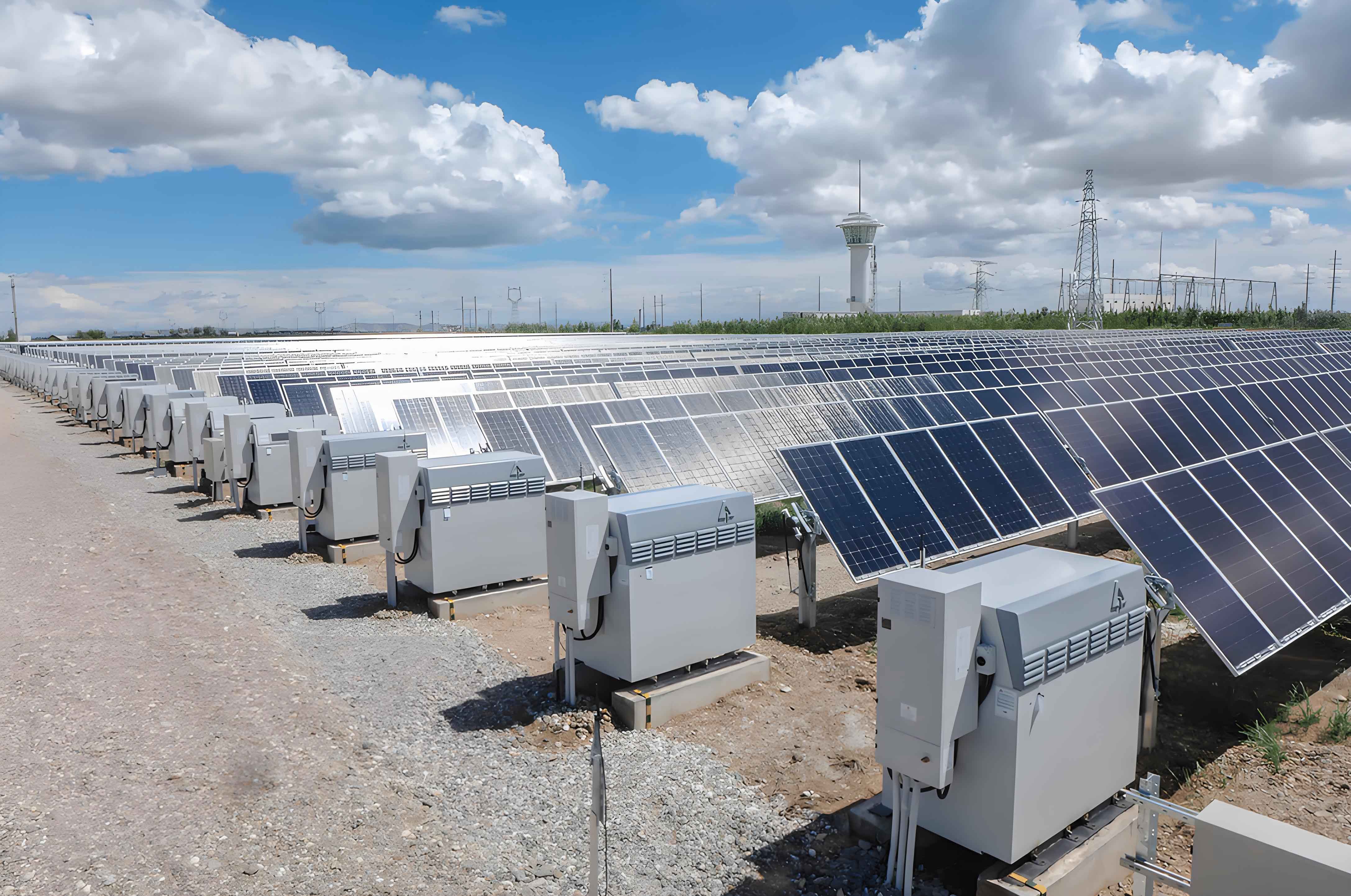
The photovoltaic power generation model utilizes the Osterwald physical prediction method, where the maximum output power forecast is derived from solar irradiance and temperature data. The power output is given by:
$$ P_{\text{pv}}(t) = K_t [1 + (T_c – T_{\text{STC}})] \frac{G}{G_{\text{STC}}} P_{\text{STC}} $$
with
$$ T_c = T + \frac{G}{800} (T_{\text{STC}} – 20) $$
where \( K_t \) is the temperature coefficient, \( T_c \) is the cell temperature during operation, \( T_{\text{STC}} \) is the cell temperature under standard test conditions, \( G \) is the actual solar irradiance, \( G_{\text{STC}} \) is the standard solar irradiance, \( P_{\text{STC}} \) is the maximum output power under standard test conditions, and \( T \) is the ambient temperature.
For wind power generation, the maximum output power forecast is calculated from predicted wind speeds. The wind turbine output power \( P_{\text{WT}} \) is expressed as:
$$ P_{\text{WT}} = \begin{cases} 0 & V < V_{\text{in}} \\ \frac{1}{2} \rho C_p \pi R^2 V^3 & V_{\text{in}} \leq V < V_r \\ P_r & V_r \leq V < V_{\text{out}} \\ 0 & V \geq V_{\text{out}} \end{cases} $$
where \( \rho \) is air density, \( C_p \) is the wind power conversion coefficient, \( R \) is the blade radius, \( V \) is the actual wind speed, \( P_r \) is the rated power, \( V_{\text{in}} \) is the cut-in speed, \( V_r \) is the rated speed, and \( V_{\text{out}} \) is the cut-out speed.
The energy storage battery model is critical for capturing degradation costs. The lifespan of the energy storage battery is defined by the total usable throughput until failure, which depends on the depth of discharge and discharge rate. The rated throughput of the energy storage battery is:
$$ A_R = L_R D_R C_R $$
where \( A_R \) is the total throughput from start to failure, \( D_R \) is the rated depth of discharge, \( C_R \) is the total energy discharged from full to empty at the rated discharge rate, and \( L_R \) is the rated cycle life at the rated depth of discharge. The actual cycle life influenced by discharge depth is fitted from experimental data:
$$ L = L_R \left( \frac{D_R}{D_A} \right)^{u_1} e^{u_0 \left( \frac{D_A}{D_R} – 1 \right)} $$
where \( L \) is the actual cycle life, \( D_A \) is the actual depth of discharge, and \( u_0 \), \( u_1 \) are fitting parameters. The equivalent discharge amount considering discharge depth is:
$$ d_R = d_{\text{act}} \left( \frac{D_R}{D_A} \right)^{u_1} e^{u_0 \left( \frac{D_A}{D_R} – 1 \right)} $$
Furthermore, the discharge rate effect is incorporated as:
$$ d_R = d_{\text{act}} \frac{C_R}{C_A} $$
where \( C_A \) is the total energy discharged at the current discharge rate. Combining both effects, the equivalent discharge per use is:
$$ d_R = d_{\text{act}} \frac{C_A}{C_R} \left( \frac{D_R}{D_A} \right)^{u_1} e^{u_0 \left( \frac{D_A}{D_R} – 1 \right)} $$
Since \( D_A = 1 – S_{\text{SOC}} \), the cost per use of the energy storage battery becomes:
$$ C_{\text{BESS}} = C_{\text{all}} \frac{d_R}{A_R} = f(S_{\text{SOC}}, d_{\text{act}}) $$
where \( C_{\text{all}} \) is the initial investment cost of the energy storage battery, \( S_{\text{SOC}} \) is the state of charge, and \( d_{\text{act}} = \Delta T x_{\text{BESS}} \) with \( x_{\text{BESS}} \) as the charging-discharging power. Thus, the cost function for the energy storage battery is:
$$ C_{\text{BESS}} = f(S_{\text{SOC}}, x_{\text{BESS}}) $$
To encourage charging of energy storage batteries with lower state of charge and reduce frequent cycling, the cost function is modified to include negative costs during charging, weighted by the current state of charge. This optimization ensures that excess power preferentially charges batteries with lower state of charge, enhancing system resilience and protecting the energy storage battery.
The bi-level optimization framework consists of an upper-level inter-microgrid dispatch and a lower-level intra-microgrid control. The upper-level objective minimizes the total operational cost of the microgrid cluster, considering dispatch losses and energy storage battery costs:
$$ \min_{x_{\text{in}}} h(x_{\text{in}}) = \sum_{i=1}^{n} \left[ f_{\text{BESS},i}(S_{\text{SOC},i}, x_{\text{BESS},i}) + \gamma_i(x_{\text{in},i}) \right] $$
with
$$ \gamma_i(x_{\text{in},i}) = \alpha_i x_{\text{in},i}^2 $$
subject to:
$$ \beta (x_{\text{DG}} + x_{\text{BESS}} – x_{\text{load}}) = x_{\text{in}} $$
$$ 0 \leq x_{\text{DG}} \leq P_{\text{DG,max}} $$
$$ \max\left( -\eta P_{\text{charge,max}}, \frac{S_{\text{SOC}} – S_{\text{SOC,max}}}{\Delta T} \right) \leq x_{\text{BESS}} \leq \min\left( P_{\text{discharge,max}}, \frac{S_{\text{SOC}} – S_{\text{SOC,min}}}{\eta \Delta T} \right) $$
where \( x_{\text{in},i} \) is the power dispatch value for microgrid \( i \) (negative for input, positive for output), \( \alpha_i \) is the loss coefficient, \( \beta \) is the dispatch efficiency, \( \eta \) is the charging-discharging efficiency, \( P_{\text{charge,max}} \) and \( P_{\text{discharge,max}} \) are maximum charging and discharging powers, and \( S_{\text{SOC,max}} \) and \( S_{\text{SOC,min}} \) are state of charge limits.
The lower-level objective minimizes the operational cost within each microgrid, including generation costs from photovoltaic and wind sources and the energy storage battery cost:
$$ \min_{x_{\text{PV}}, x_{\text{WT}}, x_{\text{BESS}}} C = \sum_{t=1}^{p} \left[ k_{\text{PV}} x_{\text{PV}} + k_{\text{WT}} x_{\text{WT}} + f_{\text{BESS}}(S_{\text{SOC}}, x_{\text{BESS}}) \right] $$
subject to:
$$ x_{\text{PV}} + x_{\text{WT}} + x_{\text{BESS}} = x_{\text{load}} + x_{\text{in}} $$
$$ 0 \leq x_{\text{PV}} \leq P_{\text{PV,max}} $$
$$ 0 \leq x_{\text{WT}} \leq P_{\text{WT,max}} $$
$$ \max\left( -\eta P_{\text{charge,max}}, \frac{S_{\text{SOC}} – S_{\text{SOC,max}}}{\Delta T} \right) \leq x_{\text{BESS}} \leq \min\left( P_{\text{discharge,max}}, \frac{S_{\text{SOC}} – S_{\text{SOC,min}}}{\eta \Delta T} \right) $$
where \( k_{\text{PV}} \) and \( k_{\text{WT}} \) are cost coefficients for photovoltaic and wind power, respectively, and \( p \) is the prediction horizon.
The optimization algorithm combines the alternating direction method of multipliers for the upper-level distributed dispatch and model predictive control for the lower-level rolling optimization. The alternating direction method of multipliers solves the upper-level problem in a distributed manner, where each microgrid iteratively updates its expected exchange power based on local information and exchanged averages. The augmented Lagrangian function is:
$$ L_\rho(x, z, \lambda) = f(x) + g(z) + \lambda^T (Ax + Bz – c) + \frac{\rho}{2} \|Ax + Bz – c\|^2 $$
The updates proceed as:
$$ x^{k+1} = \arg\min_x \left( f(x) + \frac{\rho}{2} \|Ax + Bz^k – c + u^k\|^2 \right) $$
$$ z^{k+1} = \arg\min_z \left( g(z) + \frac{\rho}{2} \|Ax^{k+1} + Bz – c + u^k\|^2 \right) $$
$$ u^{k+1} = u^k + Ax^{k+1} + Bz^{k+1} – c $$
with \( u = \lambda / \rho \). For the microgrid cluster, the update for each microgrid \( i \) is:
$$ x_{i,k+1} = \arg\min_{x_i} \left( h_i(x_i) + \frac{\rho}{2} \|x_i – x_{i,\text{ref},k+1} + u_k\|^2 \right) $$
where the reference exchange power is adjusted based on the average:
$$ x_{i,\text{ref},k+1} = x_{i,k} – \bar{x}_k, \quad \bar{x}_k = \frac{1}{n} \sum_{i=1}^{n} x_{i,k} $$
Convergence is checked via the residual:
$$ r_k = \frac{1}{n} \sum_{i=1}^{n} \|x_{i,k} – \bar{x}_k\|^2 \leq \epsilon $$
The model predictive control implements rolling optimization over a prediction horizon \( p \). At each time step, the system state is sampled, and optimal controls are computed for the horizon, but only the first control is applied. This approach handles uncertainties in renewable generation and load forecasts effectively.
For simulation, a microgrid cluster with three microgrids is considered. The distributed resource configurations are summarized in the table below.
| Configuration | Microgrid 1 | Microgrid 2 | Microgrid 3 |
|---|---|---|---|
| Wind Turbine Capacity (kW) | 500 | 500 | — |
| Photovoltaic Capacity (kW) | 300 | 500 | 500 |
| Energy Storage Battery Capacity (kWh) | 1200 | 1600 | 2000 |
| Energy Storage Battery Charging/Discharging Rate (kW) | 300 | 350 | 350 |
| Energy Storage Battery Investment Cost (10^4 CNY) | 120 | 160 | 200 |
The convergence process of the alternating direction method of multipliers shows that residuals drop below 0.01 within about 9 iterations across all time periods, indicating faster convergence compared to other distributed strategies that require 15-20 iterations. This reduces data exchange between microgrids by approximately 30%, lowering communication burden. The iterative process for exchange power at 3:00 demonstrates how microgrids balance their power needs: Microgrid 1 has surplus wind power but limits charging to protect the energy storage battery, Microgrid 2 seeks additional power for optimal charging, and Microgrid 3, without wind generation, demands power for load and battery charging. Through iterations, exchange powers converge to a global optimum.
The optimized exchange powers over a 24-hour period are obtained, and the impact of the modified energy storage battery cost function is analyzed. Comparative results before and after adjusting the cost function are presented in the following table.
| Microgrid | Before Adjustment: Energy Storage Battery Cost (CNY) | Before Adjustment: Dispatched Energy (kWh) | After Adjustment: Energy Storage Battery Cost (CNY) | After Adjustment: Dispatched Energy (kWh) |
|---|---|---|---|---|
| MG1 | 113.43 | 1385.88 | 46.23 | 995.82 |
| MG2 | 87.17 | 1266.35 | 54.17 | 822.34 |
| MG3 | 93.19 | 1694.17 | 106.28 | 1425.30 |
| Total | 293.79 | 4346.40 | 206.68 | 3243.46 |
After adjusting the energy storage battery cost function, the total energy storage battery cost decreases by 29.65%, and the dispatched energy reduces by 25.37%. Notably, energy storage batteries with lower state of charge receive more charging, enhancing their ability to handle extreme conditions, while those with higher state of charge experience fewer cycles, prolonging their lifespan. During peak load hours from 17:00 to 22:00, when photovoltaic output diminishes and demand rises, the modified strategy ensures efficient power sharing, reducing stress on transmission lines and improving system resilience.
In conclusion, I propose a bi-level distributed dispatching strategy for interconnected microgrid clusters that emphasizes the protection of the energy storage battery. By incorporating detailed models for discharge depth and rate effects, and refining the cost function to differentiate charging costs based on state of charge, the strategy optimizes the usage of the energy storage battery. The combination of the alternating direction method of multipliers and model predictive control enables efficient distributed computation with reduced communication overhead. Simulation results validate that the approach not only lowers operational costs but also enhances the reliability and longevity of the energy storage battery, making it suitable for islanded or remote microgrid applications. Future work could explore real-time implementation and integration of additional renewable sources to further improve the sustainability of microgrid clusters.