
The efficient operation of solar power plants is paramount for maximizing return on investment and contributing to clean energy goals. One of the most insidious threats to this efficiency is the formation of cracks or microfractures within individual solar panels. These defects, often invisible to the naked eye during casual inspection, can significantly degrade the electrical output of a photovoltaic (PV) module by creating resistive paths, disrupting the internal electrical circuit, and in severe cases, leading to hot spots that accelerate permanent damage. The challenge is magnified in utility-scale solar farms comprising hundreds of thousands of panels. Traditional manual inspection is not only prohibitively time-consuming, costly, and labor-intensive but is also highly subjective and prone to human error, especially for subtle crack patterns. The advent of unmanned aerial vehicles (UAVs) equipped with high-resolution cameras has revolutionized data collection, enabling the rapid acquisition of vast libraries of visible-light imagery from entire solar fields. The subsequent bottleneck, however, lies in the automated, accurate, and quantitative analysis of this image data to diagnose the health state of each solar panel.
This is where modern artificial intelligence, particularly deep learning, offers a transformative solution. Inspired by the remarkable success of deep convolutional neural networks (CNNs) in computer vision tasks like object recognition and defect detection in other industrial domains, we have developed a robust methodology for the automated identification and analysis of crack states in solar panels. Our approach leverages the fact that cracks, despite their sometimes-subtle appearance, create distinct textural and line-based features in visible light images under certain illumination conditions. We propose a deep learning-based framework that not only classifies the severity of panel cracking but also establishes a quantifiable correlation between the visual crack state and the associated electrical power generation loss. This moves beyond simple binary (cracked/not cracked) classification towards a predictive maintenance tool that can prioritize repairs based on actual performance impact.
The core of our methodology is built upon a powerful CNN architecture called the Residual Network (ResNet), further enhanced with an Attention Mechanism. To understand our model, we must first delve into the principles of these components. The primary challenge in designing very deep neural networks is the problem of vanishing gradients and network degradation, where accuracy saturates and then degrades as more layers are added. The ResNet architecture, introduced by He et al., elegantly solves this through the use of residual blocks. Instead of a stack of layers trying to directly learn an underlying mapping \( H(x) \), they learn a residual function \( F(x) = H(x) – x \). The original input \( x \) is then added to the output of the residual function via a “shortcut connection,” producing \( H(x) = F(x) + x \).
This simple reformulation has profound effects. If the optimal function is closer to an identity mapping, the solver can simply drive the weights of the residual function \( F(x) \) towards zero, making it easier to learn. This structure ensures that gradients can flow directly through the shortcut connections during backpropagation, mitigating the vanishing gradient problem. For a building block at a shallow layer \( l \) and a deeper layer \( L \), with \( \mathcal{F} \) representing the residual mapping, the feature propagation can be expressed as:
$$
x_L = x_l + \sum_{i=l}^{L-1} \mathcal{F}(x_i, W_i)
$$
During backpropagation, the gradient has a clear path:
$$
\frac{\partial \text{loss}}{\partial x_l} = \frac{\partial \text{loss}}{\partial x_L} \cdot \frac{\partial x_L}{\partial x_l} = \frac{\partial \text{loss}}{\partial x_L} \cdot \left(1 + \frac{\partial}{\partial x_l} \sum_{i=l}^{L-1} \mathcal{F}(x_i, W_i) \right)
$$
The term \( 1 \) ensures that the gradient from the deeper layer \( L \) can be propagated directly to the shallower layer \( l \) without degradation, stabilizing the training of very deep networks.
While ResNet provides the depth and stability, we incorporate an Attention Mechanism, specifically the Squeeze-and-Excitation (SE) block, to improve feature discrimination. In standard CNNs, all channel features are treated equally during fusion. However, for crack detection, some feature channels (e.g., those encoding edge or texture patterns) are more informative than others. The SE block performs channel-wise attention, adaptively recalibrating channel-wise feature responses by explicitly modeling interdependencies between channels. It operates in two steps:
- Squeeze: A global average pooling operation condenses each 2D feature map \( U_c \) (for channel \( c \)) into a channel descriptor \( z_c \), capturing the global distribution of responses.
$$
z_c = F_{sq}(u_c) = \frac{1}{H \times W} \sum_{i=1}^{H} \sum_{j=1}^{W} u_c(i, j)
$$
- Excitation: This descriptor is fed into a small, parameter-efficient neural network (typically two fully-connected layers with a bottleneck) that learns a set of channel-specific weights \( s \). This network outputs a vector of scaling factors where each element \( s_c \) corresponds to the “importance” of channel \( c \).
$$
s = F_{ex}(z, W) = \sigma(g(z, W)) = \sigma(W_2 \delta(W_1 z))
$$
Here, \( \sigma \) is the sigmoid activation, \( \delta \) is the ReLU activation, \( W_1 \in \mathbb{R}^{\frac{C}{r} \times C} \) and \( W_2 \in \mathbb{R}^{C \times \frac{C}{r}} \), with \( r \) being a reduction ratio to limit model complexity. The final output of the block is obtained by rescaling the original feature map \( U \) with the activation weights: \( \tilde{x}_c = s_c \cdot u_c \).
We embed this SE block directly into the ResNet’s residual block, creating an SE-ResNet module. This allows the network to focus its resources on the most relevant feature channels for distinguishing between different crack patterns, thereby improving both representational power and diagnostic accuracy with minimal computational overhead. The increase in parameters for an SE-ResNet50 compared to a standard ResNet50 is approximately given by:
$$
\Delta_{\text{params}} = \frac{2}{r} \sum_{s=1}^{S} N_s \cdot C_s^2
$$
Where \( S \) is the number of stages, \( N_s \) is the number of repeated blocks in stage \( s \), and \( C_s \) is the number of channels in that stage. With a typical reduction ratio \( r=16 \), the parameter increase is less than 10%, while the boost in accuracy can be significant.
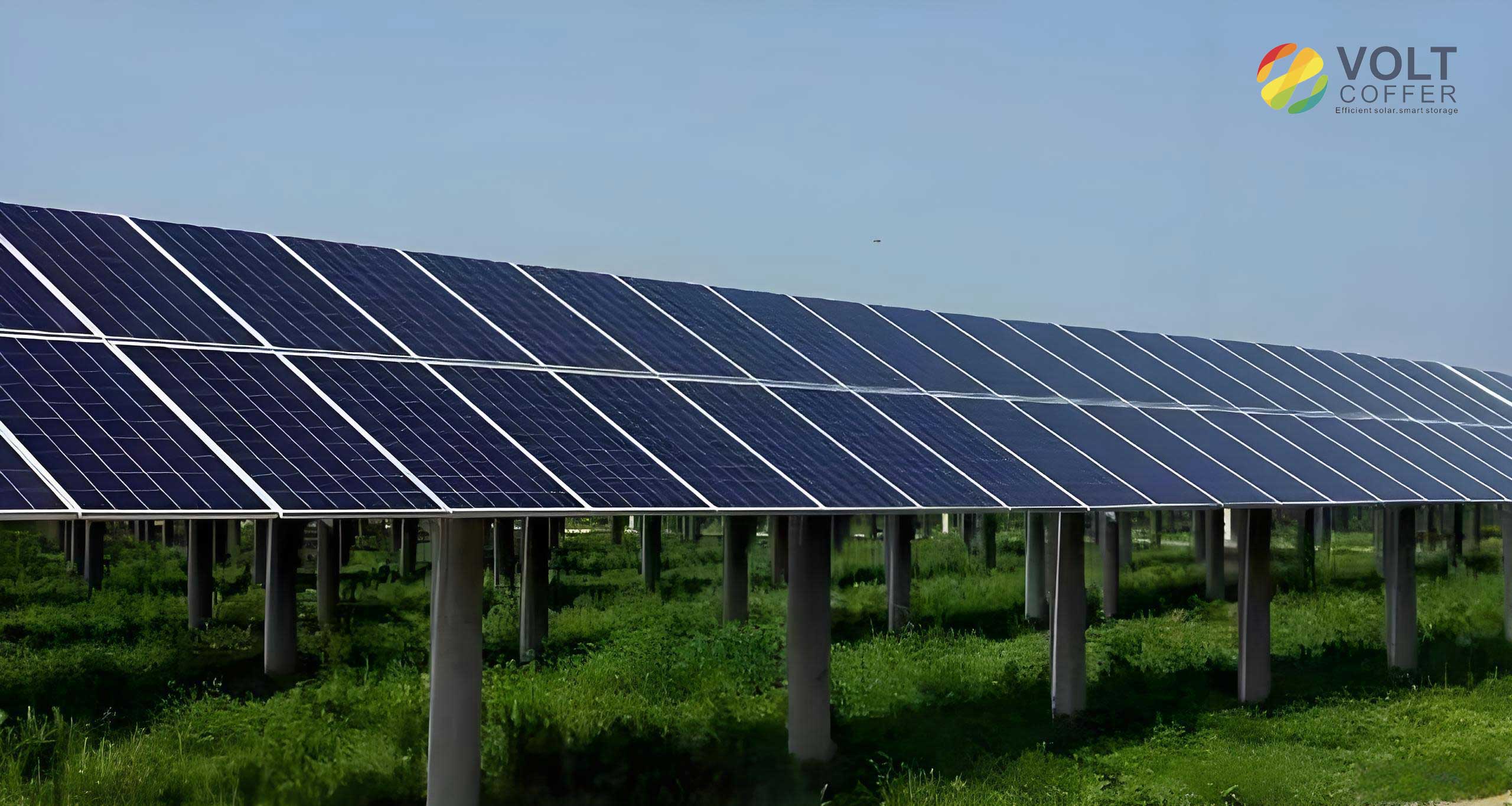
The practical application of our deep learning model hinges on high-quality, representative data. We constructed a dedicated image dataset for training and evaluation. Using a UAV-mounted high-resolution camera, we captured visible-light images of polycrystalline silicon solar panels in a operational power plant over several months. To minimize variability from lighting and sun angle, image acquisition was consistently performed between 12:00 and 14:00 local time under clear sky conditions. We focused on panels with naturally occurring and progressively worsening crack patterns, carefully selecting 2,400 images that represented a wide spectrum of crack severity. These images were then split into training and testing sets with an 80:20 ratio (1,920 images for training, 480 for testing). All images were pre-processed by resizing to a uniform 224×224 pixel resolution and normalized for model input.
The critical step for quantitative analysis was to link the visual crack state to a measurable performance metric. For each captured solar panel image, we simultaneously logged its operational data (current, voltage) and environmental data (in-plane irradiance \( G \), back-surface temperature \( T_b \)) at the moment of image capture. The power generation loss rate \( P_{loss} \) was calculated as follows:
- First, the ideal maximum power output \( P_{max, ideal} \) for an undamaged panel under the measured conditions was estimated using the panel’s rated parameters (power temperature coefficient \( \gamma \), rated efficiency \( \eta_{STC} \), area \( A \)) and a standard performance model:
$$
P_{max, ideal}(G, T_b) \approx \frac{\eta_{STC} \cdot A \cdot G}{1 + \gamma (T_b – T_{STC})}
$$
- The actual maximum power output \( P_{max, damaged} \) was derived from the logged I-V data of the cracked panel.
- The instantaneous power loss rate for that specific panel and moment was then calculated:
$$
P_{loss} = \frac{P_{max, ideal} – P_{max, damaged}}{P_{max, ideal}} \times 100\%
$$
The 2,400 images were manually annotated and grouped into six distinct classes (C0 to C5) based on their visual crack density and pattern complexity. The corresponding \( P_{loss} \) values for all images within a class were averaged to define a representative power loss label for that crack-severity class. This established the crucial ground-truth relationship for our model to learn. The statistical summary is presented in the table below.
| Crack Severity Class | Visual Description | Average Number of Cracks per Panel | Average Power Loss Rate (\( P_{loss} \)) | Number of Images |
|---|---|---|---|---|
| C0 | No visible cracks or single minor micro-crack | 0 – 1 | < 3% | 400 |
| C1 | Sparse, isolated cracks | 2 – 5 | ~ 6.5% | 400 |
| C2 | Moderate cracking, beginning to form networks | 6 – 10 | ~ 12.1% | 400 |
| C3 | Dense crack network covering significant area | 11 – 20 | ~ 18.7% | 400 |
| C4 | Severe, interconnected cracking | 21 – 35 | ~ 24.5% | 400 |
| C5 | Very severe, near-complete fragmentation | > 35 | ~ 29.0% | 400 |
Our experimental platform was configured to handle the computational demands of training deep networks. All development and simulation were conducted on a system with an Intel Core i5-9400F CPU, 16GB RAM, and an NVIDIA GeForce RTX 2060 GPU. The software stack included Windows 10, Python 3.7, PyTorch 1.1.10 deep learning framework, and CUDA 10.1 for GPU acceleration.
We implemented and compared several model architectures. The base models were ResNet-34, ResNet-50, and ResNet-101. Our proposed model was the SE-ResNet-50, which integrates the channel attention mechanism into the ResNet-50 backbone. All models were initialized with weights pre-trained on the ImageNet dataset and fine-tuned on our proprietary solar panel crack dataset. We used a cross-entropy loss function and the Adam optimizer with a scheduled learning rate. The primary evaluation metric was the Top-1 classification accuracy on the held-out test set.
The comparison results are striking and clearly demonstrate the effectiveness of our design choices. The performance and complexity metrics are summarized in the following table:
| Model Architecture | Top-1 Test Accuracy | FLOPs (G) | Number of Parameters (M) | Inference Time per Image (ms) |
|---|---|---|---|---|
| ResNet-34 | 70.42% | 3.7 | 21.8 | 15.2 |
| ResNet-50 | 83.15% | 4.1 | 25.6 | 18.7 |
| ResNet-101 | 84.26% | 7.9 | 44.5 | 32.4 |
| SE-ResNet-50 (Our Model) | 91.04% | 4.2 | 28.1 | 19.5 |
The results lead to several key conclusions. First, while ResNet-101 achieves a marginally higher accuracy (84.26%) than ResNet-50 (83.15%), it does so at more than double the computational cost (7.9 vs. 4.1 GFLOPs) and a 74% increase in parameters. This makes ResNet-50 a much more efficient and practical base architecture for potential deployment on edge devices or for processing large-scale UAV surveys. Second, and most importantly, the introduction of the Squeeze-and-Excitation attention mechanism into ResNet-50 yields a remarkable performance gain. Our SE-ResNet-50 model achieves a test accuracy of 91.04%, an improvement of nearly 8 percentage points over the vanilla ResNet-50, with only a negligible increase in FLOPs (2.4%) and parameters (9.8%). This demonstrates that the channel attention mechanism successfully guides the network to focus on the most discriminative visual features related to cracks in solar panels, such as specific texture patterns and line discontinuities, while suppressing less relevant background information.
To further analyze the model’s decision-making, we can examine the class-wise performance. The confusion matrix for our best-performing SE-ResNet-50 model reveals that most misclassifications occur between adjacent severity classes (e.g., C2 classified as C1 or C3), which is expected given the continuous nature of crack progression. The model shows very high precision and recall for the extreme classes (C0 and C5), demonstrating its strong capability in identifying both healthy and critically damaged solar panels.
In summary, we have presented a comprehensive, deep learning-based framework for the automated, quantitative assessment of crack states in photovoltaic modules. By integrating a channel attention mechanism into a robust ResNet architecture, we developed a model, SE-ResNet-50, that achieves high diagnostic accuracy (exceeding 91%) in classifying the severity of cracks from visible-light images. More significantly, our methodology establishes a direct, learned correlation between the visual appearance of a cracked solar panel and its associated electrical power generation loss. This provides a powerful tool that transcends simple defect detection. Plant operators can use this system to process thousands of UAV-captured images, automatically generate a site-wide health map, and prioritize maintenance actions based on the actual financial impact (estimated energy loss) of each faulty panel, thereby optimizing operational expenditure and maximizing energy yield.
Future work will focus on several avenues to enhance this technology further. Firstly, expanding and diversifying the dataset to include more types of solar panels (monocrystalline, thin-film), different crack origins (mechanical stress, thermal cycling), and varied environmental conditions (dust, glare, varying sun angles) will improve model robustness and generalizability. Secondly, exploring more advanced architectures like Vision Transformers (ViTs) or hybrid CNN-Transformer models may yield additional gains in accuracy. Thirdly, techniques such as network pruning and quantization can be applied to the trained SE-ResNet-50 model to reduce its size and computational footprint, making it suitable for real-time, on-board processing on drones or handheld inspection devices. Finally, integrating this image-based analysis with other data streams, such as electroluminescence imagery for sub-surface defects and time-series electrical performance data, could lead to a holistic, multi-modal health monitoring system for photovoltaic assets. This research provides a concrete and effective pathway towards intelligent, automated inspection and predictive maintenance for the global solar energy industry.