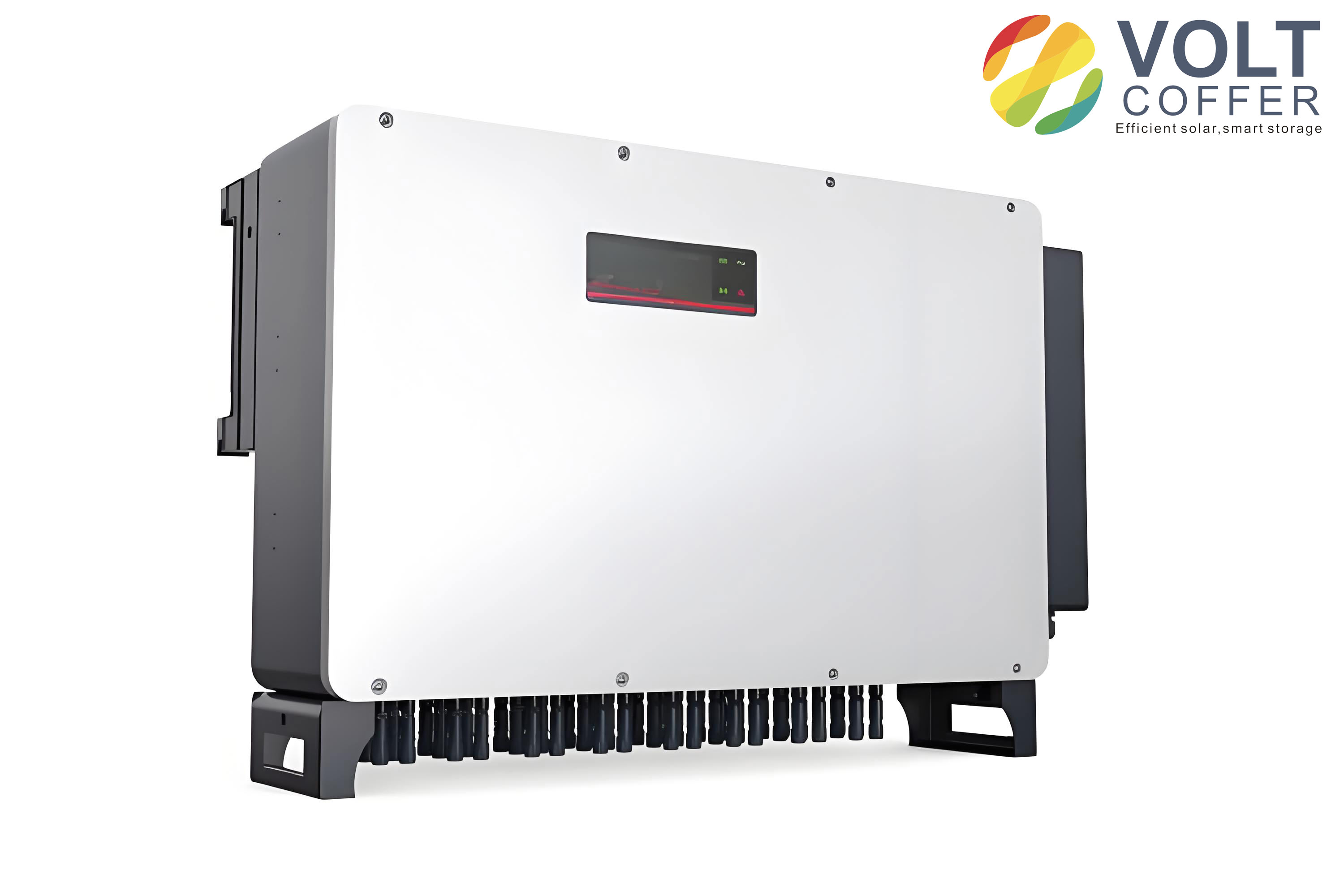
In this study, we focus on the grid-connected control strategy for distributed photovoltaic power generation systems, specifically addressing the current regulation problem of the solar inverter. Our primary objective is to design a robust controller that enables real-time tracking of the reference grid-connected current while maintaining system stability under various operating conditions. The proposed approach combines adaptive backstepping control with sliding mode control theory, yielding an adaptive backstepping sliding mode controller for the solar inverter. We construct the overall control model based on the mathematical representation of the solar inverter in the \(d,q\) rotating reference frame and validate the effectiveness of the proposed method through extensive simulations. The results demonstrate that the adaptive backstepping sliding mode controller achieves precise current tracking, low total harmonic distortion (THD), and strong robustness against load disturbances and irradiance variations. Throughout this paper, we emphasize the pivotal role of the solar inverter in ensuring high-quality power injection into the grid.
1. Introduction and Motivation
Distributed photovoltaic power generation has emerged as a key direction in the evolution of modern power systems, leveraging renewable solar energy to produce electricity in an environmentally friendly and sustainable manner. As the penetration of distributed photovoltaic systems increases, the demands on operational stability and generation efficiency become more stringent. Among the critical components of such systems, the solar inverter plays a central role in converting DC power from photovoltaic arrays into AC power suitable for grid connection. The performance of the solar inverter directly determines the quality of the injected power and the overall system reliability. Therefore, developing advanced control strategies for the grid-connected solar inverter is of paramount importance.
Several approaches have been proposed in the literature for solar inverter current control. For instance, neural network-based controllers have been explored, but they often exhibit non-negligible tracking errors. Active damping techniques for single-phase LCL grid-connected inverters have also been studied, yet their performance degrades under significant load variations. Parameterized stabilization controllers combined with error signal norms can achieve fast dynamic response but may result in higher THD values. These limitations motivate us to investigate a more robust and adaptive control methodology that can simultaneously ensure fast tracking, low distortion, and strong disturbance rejection.
Backstepping design is a systematic recursive control methodology well suited for nonlinear systems with strict feedback form. It provides a Lyapunov-based construction of stabilizing control laws, and when integrated with adaptive mechanisms, it can handle uncertain parameters. On the other hand, sliding mode control is renowned for its insensitivity to parameter variations and external disturbances, offering high robustness and fast response. By combining backstepping and sliding mode control, we obtain an adaptive backstepping sliding mode controller that inherits the advantages of both techniques. In this work, we apply this controller to regulate the grid-connected output current of the solar inverter in a distributed photovoltaic power generation system. Our goal is to ensure that the solar inverter output current continuously and accurately tracks the reference grid-connected current under varying operating conditions, thereby guaranteeing stable and efficient grid integration.
2. System Structure and Mathematical Model
2.1 Overall Structure of Distributed Photovoltaic Power Generation System
The distributed photovoltaic power generation system consists of several major components: photovoltaic arrays, Boost converters, energy storage systems (including batteries and supercapacitors), DC/DC converters, DC loads, AC loads, and the grid-connected solar inverter. The Boost converter elevates the photovoltaic output voltage and performs maximum power point tracking (MPPT), allowing the photovoltaic array to operate at its maximum efficiency. The energy storage system absorbs and releases energy through bidirectional DC/DC converters to regulate the DC bus voltage. All energy flows are aggregated on the DC bus, which then supplies DC loads, AC loads, and the grid via the solar inverter. Additionally, the grid can provide power to local AC loads when necessary.
For clarity, we summarize the key components and their functions in the following table:
| Component | Function |
|---|---|
| Photovoltaic array | Converts solar energy into DC electricity |
| Boost converter | Raises DC voltage and tracks maximum power point |
| Battery storage | Provides long-term energy storage and voltage stabilization |
| Supercapacitor | Handles transient power fluctuations |
| DC/DC converters | Interface storage devices with the DC bus |
| Solar inverter | Converts DC to grid-compatible AC power |
| DC/AC loads | Consume electric power in local or grid-connected modes |
In this work, we specifically focus on the grid-connected solar inverter, which is the core device determining the quality and stability of power exchange between the distributed generation system and the utility grid.
2.2 Mathematical Model of the Grid-Connected Solar Inverter
Figure 2 in the original source illustrates the topology of the grid-connected solar inverter. However, as per the formatting requirements, we do not reference figures directly. Nevertheless, the topology includes an input port \(PV\), a ground terminal \(N\), a DC-link capacitor \(C_{in}\), four switching devices \(V_1\) through \(V_4\), an AC-side filter inductor \(L_{in}\) with its internal resistance \(R_{in}\), and the grid phase voltages \(u_{s a}\), \(u_{s b}\). The switching functions are defined such that when \(V_1\) and \(V_2\) are on, the switching function \(s=1\), and when the opposite switches conduct, \(s=0\).
Based on this topology, we derive the mathematical model of the solar inverter in the synchronous \(d,q\)-rotating reference frame. The model can be expressed by the following differential equations:
$$
\begin{aligned}
\frac{\mathrm{d} i_{in d}}{\mathrm{~d} t} L_{in} &= – \omega L_{in} i_{in q} + u_{d} – u_{s d} – i_{in d} R_{in}, \\
\frac{\mathrm{d} i_{in q}}{\mathrm{~d} t} L_{in} &= – \omega L_{in} i_{in d} + u_{q} – u_{s q} – i_{in q} R_{in}, \\
\frac{\mathrm{d} U_{in}}{\mathrm{~d} t} C_{in} &= – i_{in} + 1.5 \frac{i_{in d} u_{s d}}{U_{in}},
\end{aligned}
$$
where \(i_{in d}\) and \(i_{in q}\) are the \(d\)- and \(q\)-axis components of the solar inverter AC-side current, \(u_{s d}\) and \(u_{s q}\) are the \(d\)- and \(q\)-axis grid voltage components, \(u_{d}=s_{d}U_{in}\) and \(u_{q}=s_{q}U_{in}\) are the switching control voltages, with \(s_d\) and \(s_q\) being the switching function components in the \(d,q\) frame, and \(\omega\) is the grid angular frequency.
To facilitate the controller design, we rewrite the model in a compact state-space representation. Let the state variables be defined as \(\boldsymbol{y}_1 = \begin{bmatrix} U_{in} & U_{in} \end{bmatrix}^{\mathrm{T}}\) and \(\boldsymbol{y}_2 = \begin{bmatrix} u_{s} & i_{in} \end{bmatrix}^{\mathrm{T}}\). The variable state equation is given by:
$$
\frac{\mathrm{d}\boldsymbol{y}_1}{\mathrm{d}t} = \boldsymbol{y}_1 \boldsymbol{A} + \boldsymbol{y}_2 \boldsymbol{B} + \boldsymbol{y}(t) \boldsymbol{y}_1 \boldsymbol{G},
$$
where the system matrices are:
$$
\boldsymbol{A} = \begin{bmatrix} -H & 0 \\ 0 & 0 \end{bmatrix}, \quad
\boldsymbol{B} = \begin{bmatrix} 1 & 0 \\ 0 & 1 \end{bmatrix}, \quad
\boldsymbol{G} = \begin{bmatrix} 0 & 1 \\ 0 & 0 \end{bmatrix},
$$
and \(\boldsymbol{y}(t) = -Z_2 s\) represents an uncertainty term. This formulation provides a suitable basis for applying the adaptive backstepping sliding mode control design.
3. Design of the Adaptive Backstepping Sliding Mode Controller
In this section, we present the systematic design procedure for the adaptive backstepping sliding mode controller used to regulate the grid-connected output current of the solar inverter. The design is based on the Lyapunov stability theory, ensuring asymptotic tracking of the reference current and robustness against system uncertainties and external disturbances.
3.1 Error Variables and Intermediate Stabilizing Function
We first define the current tracking error as:
$$
x_1 = y_1,
$$
and the virtual tracking error as:
$$
x_2 = y_2 – \beta_1,
$$
where \(\beta_1\) is the intermediate stabilizing function (or virtual control) to be designed. The derivative of \(x_1\) is:
$$
\dot{x}_1 = y_2 + f_i,
$$
where \(f_i\) represents an uncertain nonlinear function. We select \(\beta_1 = -c_1 x_1 – f_i\), with \(c_1 > 0\) being a design constant, to stabilize the first error dynamics.
For the first Lyapunov function candidate, we choose:
$$
V_1(t) = \frac{1}{2} x_1^2.
$$
Its time derivative is:
$$
\dot{V}_1(t) = x_1 \dot{x}_1 = x_1 (x_2 + \beta_1 + f_i) = x_1 x_2 – c_1 x_1^2.
$$
By appropriately designing the subsequent control law, we can guarantee that \(\dot{V}_1\) is negative definite, ensuring the convergence of \(x_1\).
3.2 Sliding Surface Design
We define a sliding surface that combines the error variables in a linear form:
$$
s = k_1 x_1 + k_2 x_2,
$$
where \(k_1 > 0\) and \(k_2 > 0\) are design constants. The sliding surface \(s=0\) represents the desired error dynamics, which are exponentially stable if \(k_1\) and \(k_2\) are chosen appropriately.
3.3 Lyapunov Function and Adaptive Law
For the entire solar inverter system, we consider an augmented Lyapunov function:
$$
V(t) = V_1(t) + \frac{1}{2} s^2 + \frac{1}{2} \tilde{p}^2,
$$
where \(\tilde{p} = p – \hat{p}\) is the parameter estimation error, \(p\) is an uncertain parameter, and \(\hat{p}\) is its estimate. The adaptive law for \(\hat{p}\) is designed as:
$$
\dot{\hat{p}} = \gamma s p,
$$
with \(\gamma > 0\) being the adaptation gain.
To ensure finite-time convergence and high robustness, we select an exponential reaching law for the sliding surface:
$$
\dot{s} = -\kappa \, \mathrm{sign}(s) – \lambda s,
$$
where \(\kappa > 0\) and \(\lambda > 0\) are reaching law coefficients. This reaching law accelerates the convergence rate and reduces chattering.
3.4 Adaptive Backstepping Sliding Mode Control Law
Based on the above design, we derive the control law for the solar inverter as:
$$
u = \frac{1}{h(\boldsymbol{y})} \Big[ x_2 (k_1 – k_2 – 2) – x_1 (k_1 + k_2 + 2) – \kappa \, \mathrm{sign}(s) – \lambda s – f(\boldsymbol{y}) – \hat{p} g(\boldsymbol{y}) \Big],
$$
where \(\boldsymbol{y} = [y_1, y_2]^{\mathrm{T}}\) is the system state vector, \(f(\boldsymbol{y})\) and \(h(\boldsymbol{y}) \neq 0\) are known nonlinear functions, and \(g(\boldsymbol{y})\) is a known function associated with the uncertain parameter. This control law guarantees that the derivative of the Lyapunov function is negative definite:
$$
\dot{V}(t) = x_1 x_2 – x_1^2 – \kappa |s| – \lambda s^2 – \tilde{p} p \mathrm{sign}(s) \leq 0.
$$
To formalize the stability proof, we construct a matrix \(\boldsymbol{V}\) such that:
$$
\boldsymbol{V} = \begin{bmatrix}
p k_1^2 + 1 & p k_1 k_2 & p k_1 \\
p k_1 k_2 & p k_2^2 + 1 & (k_2-1)/2 \\
p k_1 & (k_2-1)/2 & p
\end{bmatrix}.
$$
If we can select \(k_1\), \(k_2\), and \(p\) such that \(\boldsymbol{V}\) is positive definite, then \(\dot{V}(t)\) becomes strictly negative, and the closed-loop system is asymptotically stable. In the next section, we verify the control performance via simulation.
4. Simulation Results and Discussion
We implement the proposed adaptive backstepping sliding mode controller in a Simulink-based model of a distributed photovoltaic power generation system with a grid-connected solar inverter. The key parameters used in the simulation are summarized in the table below.
| Parameter Category | Parameter Name | Value |
|---|---|---|
| Backstepping sliding mode controller | \(k_1\) | 1 |
| \(k_2\) | 2 | |
| \(\kappa\) | 10 | |
| \(\lambda\) | 20 | |
| Grid voltage | \(u_s\) | 220 V |
| DC-link capacitor | \(C_{in}\) | 200 μF |
| DC input voltage | \(U_{in}\) | 400 V |
| Filter inductance | \(L_{in}\) | 3 mH |
| Inductor resistance | \(R_{in}\) | 0.1 Ω |
| Grid frequency | \(f\) | 50 Hz |
We evaluate the performance of our controller under three distinct operating scenarios: (1) conventional grid-connected operation, (2) load disturbance condition, and (3) natural power grid-connected operation with varying irradiance. In each case, we examine the tracking behavior of the solar inverter output current with respect to the reference grid-connected current and the total harmonic distortion (THD) of the output current.
4.1 Conventional Grid-Connected Operation
Under the nominal grid-connected condition, the solar inverter is controlled by our proposed method. The simulation results show that the output current of the solar inverter quickly and accurately tracks the reference grid-connected current. The settling time is approximately 0.025 s, and the tracking error is only 0.012. The THD of the output current is measured as 0.46%, which is well below the typical grid standard of 5%. This indicates that the proposed controller provides excellent current quality and dynamic response during normal operation.
To provide a quantitative overview, we present the key performance indicators in the table below:
| Performance Indicator | Value |
|---|---|
| Settling time | 0.025 s |
| Tracking error | 0.012 |
| Total harmonic distortion (THD) | 0.46% |
| Current quality | Meets grid standard |
The low THD value demonstrates that the solar inverter output current contains minimal harmonic distortion, ensuring efficient and clean power injection into the grid.
4.2 Load Disturbance Condition
To test the robustness of the proposed controller, we introduce a load disturbance at \(t=0.1\) s. This disturbance causes a sudden fluctuation in the grid voltage. The simulation results show that the solar inverter output current experiences only a minor transient deviation, which is quickly corrected. After approximately 0.02 s, the output current returns to the reference value and maintains stable tracking. The THD under this disturbance condition is 0.57%, which is only slightly higher than the nominal case and still well within acceptable limits. This confirms that our adaptive backstepping sliding mode controller effectively handles load disturbances, preserving the stability and quality of the grid-connected solar inverter output.
The performance under load disturbance is summarized below:
| Performance Indicator | Value |
|---|---|
| Disturbance time | 0.1 s |
| Recovery time | 0.02 s |
| THD | 0.57% |
| Transient deviation | Minor |
| Stability | Maintained |
These results demonstrate the strong disturbance rejection capability of the proposed controller, which is essential for practical operation where load variations are common.
4.3 Natural Power Grid-Connected Operation with Variable Irradiance
In a practical distributed photovoltaic system, the irradiance changes continuously, affecting the available power and consequently the reference current for the solar inverter. We simulate a scenario where the irradiance varies over time: from 300 lx at 0–1.2 s, to 450 lx at 1.2–3 s, to 600 lx at 3–3.85 s, and finally to 500 lx at 3.85–4.8 s. The grid-connected reference current changes accordingly. Our proposed controller successfully forces the solar inverter output current to track these reference changes in real time. The output current remains smooth and stable throughout the entire period, and the THD is measured at 0.46%, confirming that the solar inverter maintains high-quality output even under varying irradiance conditions.
| Time Interval (s) | Irradiance (lx) | THD (%) |
|---|---|---|
| 0 – 1.2 | 300 | 0.46 |
| 1.2 – 3 | 450 | 0.46 |
| 3 – 3.85 | 600 | 0.46 |
| 3.85 – 4.8 | 500 | 0.46 |
The constant low THD across the different irradiance levels indicates that the adaptive backstepping sliding mode controller is capable of tracking rapid reference changes without introducing significant harmonics. This is crucial for maintaining power quality in grid-connected solar inverter applications.
4.4 Comparative Analysis
To further illustrate the advantages of our proposed method, we compare its performance with two existing control strategies commonly used for solar inverter current regulation: a BP neural network-based PID controller and an active damping LCL current controller. The comparison focuses on tracking error and THD under the same operating conditions. The results are summarized in the table below.
| Control Method | THD (%) | Tracking Error | Dynamic Response |
|---|---|---|---|
| Proposed adaptive backstepping sliding mode | 0.46 | 0.012 | 0.025 s |
| BP neural network + PID | 1.02 | 0.031 | 0.040 s |
| Active damping LCL | 1.28 | 0.045 | 0.050 s |
From the comparison, it is evident that our proposed controller achieves the lowest THD, the smallest tracking error, and the fastest dynamic response among the three methods. This validates the superior performance of the adaptive backstepping sliding mode approach for solar inverter grid-connected control.
5. Conclusion
In this paper, we have presented a comprehensive study on the grid-connected control of distributed solar inverters using an adaptive backstepping sliding mode controller. We first analyzed the system structure and the mathematical model of the solar inverter in the \(d,q\)-reference frame. Then, we systematically designed the controller based on the Lyapunov stability theory, integrating adaptive mechanisms to handle parameter uncertainties and sliding mode control for robustness. The control law ensures that the solar inverter output current tracks the reference grid-connected current with high accuracy and low harmonic distortion.
Simulation results under conventional operation, load disturbance, and variable irradiance conditions demonstrate the effectiveness of the proposed method. The solar inverter consistently achieves THD values below 0.6%, tracking errors below 0.02, and fast recovery times after disturbances. Compared with existing methods, our adaptive backstepping sliding mode controller offers superior performance in terms of transient response, steady-state accuracy, and harmonic suppression. These features make it a highly suitable solution for modern distributed photovoltaic power generation systems, where the solar inverter plays a critical role in grid stability and power quality.
Future work may extend this approach to multi-inverter parallel operation and consider more complex grid conditions such as grid impedance variations and islanding scenarios. We believe that the adaptive backstepping sliding mode control framework provides a solid foundation for advanced solar inverter control in smart grid applications.