
In this paper, we investigate the optimal configuration of battery energy storage systems (BESS) in distribution networks under the influence of wind and solar uncertainty. The work focuses on reducing the daily average network loss while accounting for the stochastic nature of renewable generation. We establish wind and photovoltaic probability models, construct a joint wind–solar output function using the Frank Copula function, and generate representative scenarios through Latin Hypercube Sampling and K-means clustering. To solve the capacity allocation problem, we propose an improved sand cat swarm optimization (ISCSO) algorithm that integrates adaptive dynamic parameters, a sparrow search exploration mechanism, and Lévy flight. The proposed method is tested on the IEEE-33 node distribution system with different numbers of BESS. Simulation results show that the ISCSO algorithm outperforms the original SCSO algorithm in minimizing the daily average network loss, and the optimal BESS capacity configuration is obtained. This study confirms that the improved algorithm is an effective and practical approach for planning energy storage systems in renewable-rich distribution networks.
1 Introduction
With the rapid development of the global economy and technology, the demand for energy and its consumption has increased significantly. The excessive use of fossil fuels has caused serious environmental issues, and renewable energy sources such as wind and solar have become a turning point in the power industry. However, wind and solar power are highly dependent on weather conditions, and their output has strong randomness, volatility, and intermittency. When large amounts of wind and solar power are integrated into the distribution network, the stability of the power grid can be adversely affected. To mitigate these problems, battery energy storage systems have attracted considerable attention. An energy storage system can perform energy time-shifting and power regulation, effectively smoothing the fluctuations caused by renewable generation and improving the reliability and economy of the distribution network. Nevertheless, the cost of energy storage batteries is relatively high, and an unreasonable placement or capacity configuration may lead to voltage violations, increased network losses, and wasted investment. Therefore, optimizing the location and sizing of energy storage systems is an important research topic.
The uncertainty associated with wind and solar output has been studied by many researchers. Common methods include chance-constrained programming, stochastic optimization, and scenario analysis. In this work, we adopt the scenario analysis method. We first construct probability models for wind speed and solar irradiance, then use a Copula function to model the joint distribution of wind and solar output. The Latin Hypercube Sampling (LHS) method is employed to generate a large number of scenarios, and the K-means clustering algorithm is used to reduce the number of scenarios while preserving typical characteristics. This approach effectively captures the uncertainty of renewable generation for subsequent energy storage system planning.
Optimization algorithms play a crucial role in solving the energy storage system configuration problem. Heuristic algorithms such as particle swarm optimization, gray wolf optimization, whale optimization, and sand cat swarm optimization (SCSO) have been widely applied. The SCSO algorithm, proposed recently, has shown advantages in fast convergence and strong search capability. However, it also suffers from weak global exploration and a tendency to fall into local optima in the later iterations. To overcome these drawbacks, we propose an improved sand cat swarm optimization (ISCSO) algorithm. The improvements include an adaptive dynamic parameter, a sparrow search exploration strategy, and the Lévy flight mechanism. The enhanced algorithm is tested on benchmark functions and then applied to the BESS capacity optimization model established in this paper.
2 Applications and Impacts of Distributed Energy Storage Systems
2.1 Application Scenarios
Distributed energy storage systems are widely used in user-side, grid-side, and generation-side applications. On the user side, energy storage systems are mainly used for peak-valley price arbitrage and demand charge management. By charging during low-price periods and discharging during high-price periods, users can reduce their electricity bills and help the grid perform peak shaving. On the grid side, energy storage systems can alleviate line congestion, postpone transmission and distribution upgrades, and provide grid frequency regulation. On the generation side, energy storage systems facilitate the integration of renewable energy and support peak-valley adjustment. The role of an energy storage system in these scenarios is critical for maintaining power balance and improving system efficiency.
2.2 Classification of Distributed Energy Storage
| Category | Type | Typical Applications |
|---|---|---|
| Physical storage | Pumped hydro, compressed air, flywheel | Large-scale energy management, frequency regulation |
| Electrochemical storage | Lead-acid battery, lithium-ion battery | Renewable integration, peak shaving |
| Other storage | Supercapacitor, hydrogen storage | Fast response, long-duration storage |
2.3 Battery Energy Storage System Structure
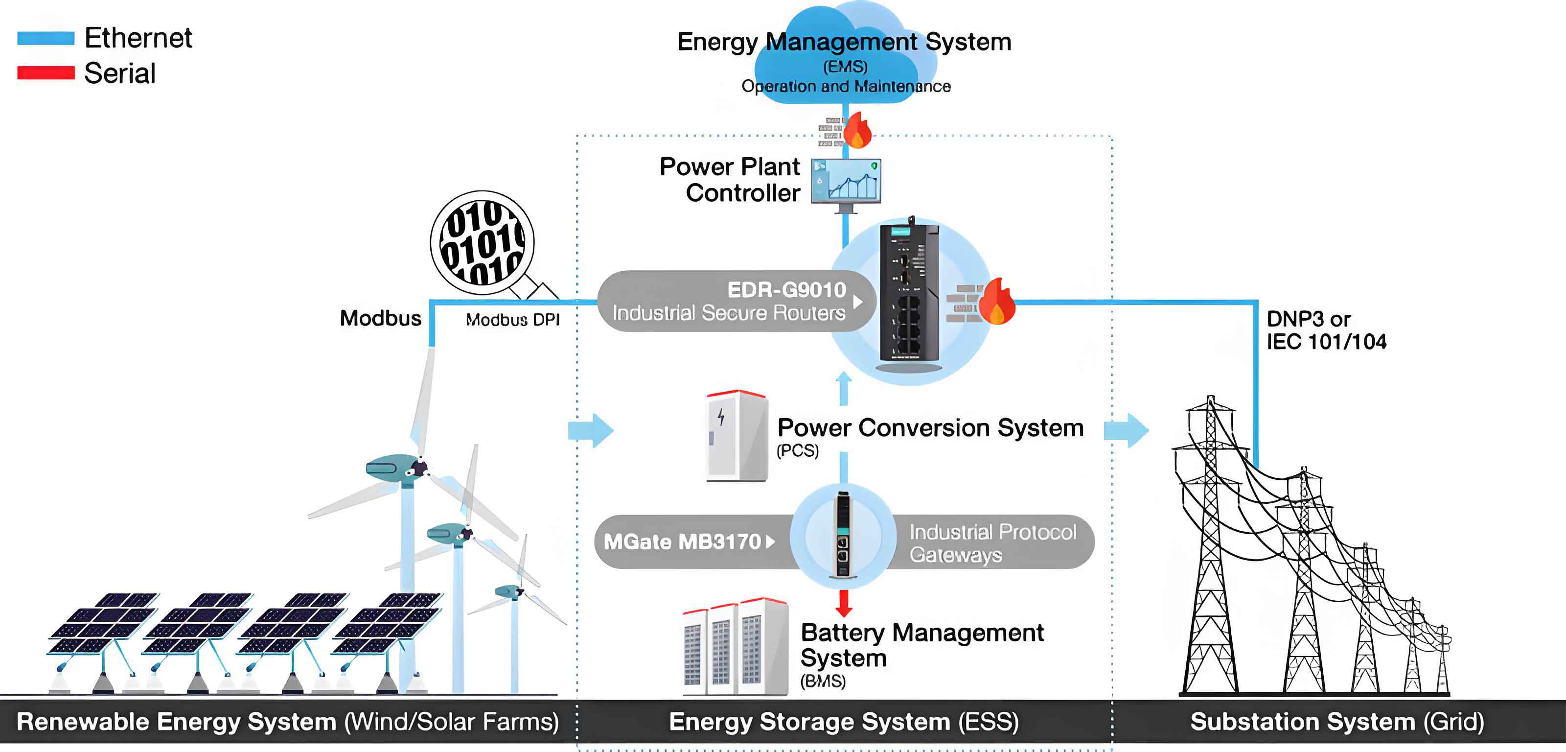
A battery energy storage system consists of four main components: the battery system (BS), the power conversion system (PCS), the battery management system (BMS), and the energy management system (EMS). The battery system is the core energy storage part, composed of multiple cells connected in series and parallel to achieve the desired capacity. The PCS acts as an interface between the battery and the grid, controlling the charging and discharging process and converting between DC and AC. The BMS monitors the state of each cell, ensuring safety, balancing, and protecting the battery from overcharge or over-discharge. The EMS manages the overall control strategy and optimizes the operation of the energy storage system according to the grid requirements. The following figure illustrates a typical battery energy storage system architecture.
2.4 Impact of BESS on Distribution Network Voltage and Losses
The connection of an energy storage system to the distribution network can influence the nodal voltages and power losses. When the BESS is charging, it behaves as a load, which decreases the voltage at the connected node. When discharging, it behaves as a generator, raising the voltage. The voltage drop between two adjacent nodes in the distribution network can be expressed as:
\[
\Delta U = \frac{P_2 R_1 + Q_2 X_1}{U_2} + j\frac{P_2 X_1 – Q_2 R_1}{U_2}
\]
Ignoring the vertical component in distribution networks, the voltage difference is approximated by:
\[
U_2 = U_1 + \frac{P_2 R_1 + Q_2 X_1}{U_2}
\]
When a BESS is installed at the downstream node, the relation becomes:
\[
U_2 = U_1 + \frac{(P_2 + P_{BESS})R_1 + (Q_2 + Q_{BESS})X_1}{U_2}
\]
where \(P_{BESS}>0\) indicates charging and \(P_{BESS}<0\) indicates discharging. The same principle can be extended to any two nodes in the network. If the BESS is charged, the voltage difference between upstream and downstream nodes increases, lowering the overall voltage profile. Conversely, discharging increases the voltage. Therefore, the location and capacity of an energy storage system must be optimized to avoid adverse voltage deviations.
In addition, the energy storage system changes the power flow distribution, which directly affects the network losses. By charging during off-peak hours and discharging during peak hours, the BESS can smooth the load curve and reduce the losses caused by high current flows. Both active and reactive power regulation capabilities contribute to loss reduction. A well-planned energy storage system is therefore an effective means to improve the economic operation of distribution networks.
3 Uncertainty Analysis and Scenario Generation
3.1 Methods for Uncertainty Handling
Two main approaches are used to handle the uncertainty of renewable energy output: stochastic programming and robust optimization. In this work, we adopt the scenario-based method, which belongs to the stochastic programming category. Scenario generation and scenario reduction are the two key steps. We use the Latin Hypercube Sampling (LHS) method for scenario generation and the K-means clustering algorithm for scenario reduction.
3.2 Wind Power Probability Model
Wind power output is a function of wind speed. The relationship between wind speed \(v\) and the output power \(P_w\) of a wind turbine is given by:
\[
P_w(v)=
\begin{cases}
0, & v < v_{ci} \text{ or } v > v_{co} \\
\sigma_w + \eta_w v, & v_{ci} \le v \le v_r \\
P_r, & v_r \le v \le v_{co}
\end{cases}
\]
where \(v_{ci}\), \(v_r\), and \(v_{co}\) are the cut-in, rated, and cut-out wind speeds, respectively, and \(P_r\) is the rated power. The coefficients \(\sigma_w\) and \(\eta_w\) are given by:
\[
\sigma_w = -\frac{P_r v_{ci}}{v_r – v_{ci}}, \qquad \eta_w = \frac{P_r}{v_r – v_{ci}}
\]
To model the randomness of wind speed, the Weibull distribution is commonly used:
\[
f(v)=\frac{k}{c}\left(\frac{v}{c}\right)^{k-1}\exp\left[-\left(\frac{v}{c}\right)^k\right], \quad v>0
\]
where \(k\) is the shape parameter and \(c\) is the scale parameter. They can be estimated from the mean \(\mu_{WT}\) and standard deviation \(\sigma_{WT}\) of wind speed:
\[
k = \left(\frac{\sigma_{WT}}{\mu_{WT}}\right)^{-1.086}, \qquad c = \frac{\mu_{WT}}{\Gamma(1+1/k)}
\]
The Weibull distribution is a parametric model with a fixed functional form. To obtain more accurate fitting, a non-parametric kernel density estimation is adopted:
\[
\hat{f}_w(v) = \frac{1}{nh}\sum_{i=1}^{n} K\left(\frac{v-v_i}{h}\right)
\]
where \(n\) is the number of samples, \(h\) is the bandwidth, and \(K(\cdot)\) is the kernel function. The total active power of a wind farm with \(M\) turbines is:
\[
P_w = \sum_{i=1}^{M} P_{w,i}
\]
3.3 Photovoltaic Probability Model
The output power of a photovoltaic (PV) array is determined by the solar irradiance \(L\) and the effective area \(A_s\):
\[
P_s = \eta_s L A_s
\]
where \(\eta_s\) is the photoelectric conversion efficiency. The randomness of solar irradiance is often described by a Beta distribution:
\[
f(L)=\frac{\Gamma(\alpha+\beta)}{\Gamma(\alpha)\Gamma(\beta)}\left(\frac{L}{L_{max}}\right)^{\alpha-1}\left(1-\frac{L}{L_{max}}\right)^{\beta-1}
\]
where \(L_{max}\) is the maximum irradiance, and \(\alpha\), \(\beta\) are shape parameters. They are derived from the mean \(\mu\) and standard deviation \(\sigma\) of irradiance:
\[
\alpha = \mu\left(\frac{\mu(1-\mu)}{\sigma^2}-1\right), \qquad \beta = (1-\mu)\left(\frac{\mu(1-\mu)}{\sigma^2}-1\right)
\]
Similar to wind speed, a non-parametric kernel density estimation can be used for a better fit:
\[
\hat{f}_s(P_s) = \frac{1}{nh}\sum_{i=1}^{n} K\left(\frac{P_s-P_{s,i}}{h}\right)
\]
3.4 Joint Wind–Solar Output Modeling via Copula Functions
A Copula function is a useful tool for modeling the dependence structure between random variables. For two random variables \(x\) and \(y\) with marginal distribution functions \(F(x)\) and \(F(y)\), the joint distribution function \(T(x,y)\) can be expressed as:
\[
T(x,y) = C(F(x), F(y))
\]
where \(C\) is the Copula function. The corresponding joint probability density function is:
\[
t(x,y) = c(F(x),F(y)) f(x) f(y)
\]
To measure the nonlinear dependence, the Kendall rank correlation coefficient is used:
\[
\rho = P[X_1-X_2)(Y_1-Y_2)>0] – P[(X_1-X_2)(Y_1-Y_2)<0]
\]
In this paper, we choose the Frank Copula function from the Archimedean family, which provides a satisfactory fit for wind and solar output data. The Frank Copula distribution function is:
\[
C(u_1,u_2;\theta) = -\frac{1}{\theta}\ln\left[1+\frac{(e^{-\theta u_1}-1)(e^{-\theta u_2}-1)}{e^{-\theta}-1}\right]
\]
where \(\theta \in (-\infty,0)\cup(0,+\infty)\). The relationship between \(\theta\) and Kendall’s rank correlation coefficient is:
\[
\rho = 1 + \frac{4}{\theta}\left[\frac{1}{\theta}\int_0^\theta \frac{x}{e^x-1}dx -1\right]
\]
Consequently, the joint wind–solar output density function is written as:
\[
t(P_w,P_s) = \frac{\theta e^{-\theta(F(P_w)+F(P_s))}(e^{-\theta}-1) f(P_w) f(P_s)}{\left[(e^{-\theta}-1)+(e^{-\theta F(P_w)}-1)(e^{-\theta F(P_s)}-1)\right]^2}
\]
3.5 Scenario Generation and Reduction
Based on the selected Copula function, the Latin Hypercube Sampling method is used to generate a large number of wind and solar output scenarios. The procedure is as follows:
- Collect hourly wind speed and solar irradiance data for a typical region.
- Estimate the marginal distribution and density functions of wind and solar output using non-parametric kernel density estimation.
- Construct the joint distribution function using the Frank Copula function.
- Divide the wind–solar output curves into subintervals and apply inverse sampling to generate \(m\) scenarios.
To reduce the computational burden, the K-means clustering algorithm is used. Suppose there are \(n\) samples, each with \(p\) features. The sample set is denoted as:
\[
x_i = (x_{i1}, x_{i2}, \ldots, x_{ip}), \quad i=1,2,\ldots,n
\]
The initial cluster centers are denoted as:
\[
z_j = (z_{j1}, z_{j2}, \ldots, z_{jp}), \quad j=1,2,\ldots,k
\]
For each sample, the Euclidean distance to each cluster center is calculated:
\[
d_{ij} = \sqrt{\sum_{m=1}^{p} (x_{im} – z_{jm})^2}
\]
The steps are: (1) randomly select \(k\) initial centers; (2) assign each sample to the closest center; (3) recompute each cluster center as the mean of its members; (4) repeat until convergence. The final cluster centers represent the typical scenarios, and the probability of each scenario is obtained from the proportion of samples in that cluster.
3.6 Verification with Real Data
We use one year of hourly wind speed and solar irradiance data from a certain region to validate the proposed uncertainty models. The Weibull distribution and the non-parametric kernel density method are fitted to wind speed data. The fitting parameters are listed in the following table.
| Method | Parameter | Value |
|---|---|---|
| Weibull | Shape \(k\) | 4.2754 |
| Weibull | Scale \(c\) | 2.3749 |
| Kernel density | Kernel function | Gaussian |
| Kernel density | Bandwidth \(h\) | 0.3143 |
The goodness of fit is evaluated using the Pearson chi-square statistic \(\chi^2\), the mean absolute percentage error (MAP), and the root mean square error (RMS). The formulas are:
\[
\chi^2 = \sum_{i=1}^{k} \frac{(X_i – Y_i)^2}{Y_i}
\]
\[
MAP = \frac{1}{k}\sum_{i=1}^{k}\left|\frac{P_{w,i}-P_{s,i}}{P_{s,i}}\right|\times 100\%
\]
\[
RMS = \sqrt{\frac{1}{k}\sum_{i=1}^{k}(P_{w,i}-P_{s,i})^2}
\]
The fitting results are summarized below.
| Distribution | \(\chi^2\) | MAP | RMS |
|---|---|---|---|
| Weibull | 16.328 | 13.67% | 0.0283 |
| Kernel density | 6.749 | 7.55% | 0.0091 |
For solar irradiance, the Beta distribution and non-parametric kernel density estimation are compared. The fitting parameters are listed below.
| Method | Parameter | Value |
|---|---|---|
| Beta | \(\alpha\) | 0.417 |
| Beta | \(\beta\) | 1.763 |
| Kernel density | Kernel function | Gaussian |
| Kernel density | Bandwidth \(h\) | 0.034 |
| Distribution | \(\chi^2\) | MAP | RMS |
|---|---|---|---|
| Beta | 16.328 | 13.67% | 0.0283 |
| Kernel density | 6.749 | 7.55% | 0.0091 |
At a significance level of 0.05 and 12 degrees of freedom, the critical \(\chi^2\) value is 20.026. Both methods pass the test, but the kernel density method has smaller \(\chi^2\) values and errors, indicating a better fit. Therefore, the non-parametric kernel density method is selected for modeling both wind speed and solar irradiance.
Using the Frank Copula function and LHS, we generate 800 wind and solar output scenarios. Then, K-means clustering reduces them to 10 typical scenarios. The probability of each reduced scenario is given in the following table.
| Scenario | 1 | 2 | 3 | 4 | 5 | 6 | 7 | 8 | 9 | 10 |
|---|---|---|---|---|---|---|---|---|---|---|
| Probability | 0.100 | 0.110 | 0.090 | 0.1025 | 0.123 | 0.109 | 0.090 | 0.090 | 0.069 | 0.012 |
4 Optimal Configuration Model and Improved Algorithm
4.1 Objective Function
To evaluate the effect of an energy storage system on the distribution network, we minimize the daily average network loss. The objective function is defined as:
\[
\min f = \sum_{s=1}^{PN} P(s) \cdot f_1(s)
\]
where \(PN\) is the number of typical scenarios, \(P(s)\) is the probability of scenario \(s\), and \(f_1(s)\) is the daily network loss under scenario \(s\). The daily network loss is calculated by:
\[
f_1 = \min \sum_{t=1}^{T} \sum_{b=1}^{n} I_b^2(t) R_b
\]
where \(T\) is the time horizon (24 h), \(n\) is the number of branches, \(I_b(t)\) is the current of branch \(b\) at time \(t\), and \(R_b\) is the resistance of branch \(b\).
4.2 Constraints
The following constraints must be satisfied during the optimization.
Node voltage limits:
\[
V_L < V_j < V_H, \quad V_H \le V_{MAX}
\]
Power balance constraints:
\[
\sum_{k=1}^{n_n} P_{E,k}(t) = \sum_{k=1}^{n} \left( P_{pv,k}(t) + P_{pw,k}(t) + P_{g,k}(t) \right)
\]
BESS power and state-of-charge (SOC) constraints:
\[
P_{BESS}^{min} \le P_{BESS} \le P_{BESS}^{max}
\]
\[
SOC_{min} \le SOC(t) \le SOC_{max}
\]
Energy balance constraint for each BESS:
\[
\int_{0}^{T} P_{BESS}(t)\, dt = 0
\]
4.3 Sand Cat Swarm Optimization
The sand cat swarm optimization (SCSO) algorithm is a nature-inspired metaheuristic based on the hunting behavior of sand cats. The algorithm has two main phases: exploration and exploitation. The population is initialized randomly:
\[
X_i = d_b + rand(0,1) \cdot (u_b – d_b)
\]
The sensitivity range \(r_G\) is defined as:
\[
r_G = S_M – \frac{S_M \times t_i}{t_{max}}
\]
where \(S_M = 2\), \(t_i\) is the current iteration, and \(t_{max}\) is the maximum number of iterations. Each cat has a random sensitivity \(r = r_G \times rand(0,1)\). In the exploration phase, the position is updated by:
\[
X(t+1) = r \cdot X_{bc}(t) – rand(0,1) \cdot X_c(t)
\]
In the exploitation phase, the position is updated based on the distance between the best position and the current position:
\[
X_{rnd} = rand(0,1) \cdot (X_b(t) – X_c(t))
\]
\[
X(t+1) = X_b(t) – r \cdot \cos(\theta) \cdot X_{rnd}
\]
The balance parameter \(R\) controls the transition between exploration and exploitation:
\[
R = 2 \times r_G \times rand(0,1) – r_G
\]
The position update rule is:
\[
X(t+1)=
\begin{cases}
X_b(t) – r \cdot \cos(\theta) \cdot X_{rnd}, & R \le 1 \\
r \cdot X_{bc}(t) – rand(0,1) \cdot X_c(t), & R > 1
\end{cases}
\]
4.4 Improved Sand Cat Swarm Optimization (ISCSO)
The original SCSO algorithm has some drawbacks. The linear sensitivity range may not provide a good balance between exploration and exploitation, and the algorithm can become trapped in local optima. Therefore, we propose three improvements.
1. Adaptive dynamic parameter: Instead of the linear decrease of \(r_G\), we adopt a nonlinear adaptive strategy:
\[
r_G = S_M \left(1 – \ln\left(1 + (e-1)\frac{iter}{MaxIt}\right)\right)
\]
where \(iter\) is the current iteration number and \(MaxIt\) is the maximum iteration count. This makes the decline slow at the beginning, allowing a thorough global search, and faster at the end to improve convergence.
2. Sparrow search exploration strategy: In the exploration phase, we incorporate the discoverer position update mechanism from the sparrow search algorithm:
\[
x_i^{t+1} =
\begin{cases}
x_i^{t} \exp\left(-\frac{i}{\alpha \cdot MaxIt}\right), & R_2 < ST \\
x_i^{t} + Q \cdot L, & R_2 \ge ST
\end{cases}
\]
where \(\alpha\) is a random number in \([0,1]\), \(R_2\) is the alarm value, \(ST\) is the safety threshold, \(Q\) is a random number following the standard normal distribution, and \(L\) is a row vector of ones with the same dimension as \(x_i\).
3. Lévy flight mechanism: To prevent the algorithm from missing promising solutions, we add Lévy flight random perturbation:
\[
X(t+1) = X(t) + \alpha \cdot Levy(\lambda)
\]
where \(\alpha\) is the step size factor (usually 0.01). The Lévy distribution can be simulated using Mantegna’s algorithm:
\[
Levy(\lambda) = \frac{\mu}{|\nu|^{1/\beta}}
\]
where \(\mu \sim N(0,\sigma_\mu^2)\), \(\nu \sim N(0,\sigma_\nu^2)\), and
\[
\sigma_\mu = \left[\frac{\Gamma(1+\beta)\sin(\pi\beta/2)}{\Gamma((1+\beta)/2)\beta 2^{(\beta-1)/2}}\right]^{1/\beta}, \quad \sigma_\nu = 1
\]
Here \(\beta\) is a constant, usually 1.5. The improved algorithm is named ISCSO.
4.5 Benchmark Test
To verify the performance of ISCSO, we compare it with SCSO, DBO, GWO, WOA, and PSO on two benchmark functions: a unimodal function and a multimodal function. The population size is 100 and the maximum number of iterations is 200.
| Function | Expression | Dimension | Range | Theoretical optimum |
|---|---|---|---|---|
| Unimodal F1 | \(F_1(x)=\sum_{i=1}^{n} x_i^2\) | 30 | [-100,100] | 0 |
| Multimodal F10 | \(F_{10}(x)=\sum_{i=1}^{n}[x_i^2 – 10\cos(2\pi x_i)+10]\) | 30 | [-5.12,5.12] | 0 |
The convergence curves show that ISCSO converges faster and reaches lower objective values than the compared algorithms. For the unimodal function, ISCSO achieves the theoretical optimum with a much smaller number of iterations. For the multimodal function, ISCSO also obtains better global search capability and avoids premature convergence. These results confirm the effectiveness and superiority of the proposed improvements for the energy storage system optimization problem.
5 Simulation Experiments and Results
5.1 System and Parameters
The proposed method is tested on the IEEE-33 node distribution system. The system has 33 nodes and 32 branches. The branch parameters are listed in Table 5. A photovoltaic generation unit is connected at node 10, and a wind farm is connected at node 22. The base voltage is 12.66 kV and the base power is 10 MVA. The typical wind–solar scenarios are obtained from the previous section. The parameters of the ISCSO algorithm are set as follows.
| Parameter | Value |
|---|---|
| Population size | 100 |
| Maximum iterations | 200 |
| Sensitivity \(S_M\) | 2 |
| Safety threshold \(ST\) | 0.8 |
5.2 Solving Procedure
The optimization procedure is as follows:
- Generate an initial population of sand cats, where each individual represents a possible BESS capacity and location scheme.
- Calculate the fitness value of each individual using the objective function defined in Section 4.1.
- Update the sensitivity range with the adaptive dynamic parameter.
- Based on the value of \(R\), switch between the improved exploration and exploitation phases.
- Apply the Lévy flight mechanism to selected individuals to increase diversity.
- Update the global best position and check the stopping criterion.
- Output the optimal BESS configuration.
5.3 Results and Analysis
We simulate the connection of 1, 2, 3, and 4 BESS units to the IEEE-33 system. Both SCSO and ISCSO are used to solve the optimization model. The minimum daily average network loss for each case is listed in the following table.
| Number of BESS | Algorithm | BESS locations | Capacity (kWh) | Minimum loss (kW) |
|---|---|---|---|---|
| 1 | SCSO | 12 | 125.7 | 186.427 |
| 2 | SCSO | 18, 29 | 179.3, 184.6 | 186.276 |
| 3 | SCSO | 6, 13, 17 | 101, 171.3, 163.4 | 186.208 |
| 4 | SCSO | 2, 3, 17, 25 | 57, 73.8, 163.4, 143.2 | 186.548 |
| 1 | ISCSO | 28 | 161.6 | 181.250 |
| 2 | ISCSO | 8, 32 | 123.4, 165 | 180.498 |
| 3 | ISCSO | 7, 14, 24 | 161.2, 178.4, 195.3 | 178.240 |
| 4 | ISCSO | 5, 8, 16, 25 | 98, 134.7, 175.3, 165.9 | 179.560 |
From the results, the daily network loss is minimized when three BESS units are installed. The ISCSO algorithm always gives a lower minimum loss than the original SCSO, which demonstrates that the improved algorithm is more effective in solving the energy storage system configuration problem. Moreover, the output power profiles of the BESS for different cases show that the charging and discharging states follow the load curve and the renewable output pattern. In particular, for the three-BESS case, the ISCSO solution results in higher power utilization (up to 40 kW) while still achieving a lower network loss than the SCSO solution. This indicates that the improved algorithm can not only reduce the daily average network loss but also improve the utilization efficiency of the energy storage system.
5.4 Optimal Capacity Configuration of BESS
Based on the ISCSO solution with three BESS units, the optimal nodes are 7, 14, and 24, with capacities of at least 161 kWh, 178 kWh, and 195 kWh, respectively. We choose a practical lithium iron phosphate battery cell with a rated voltage of 3.2 V and a capacity of 200 Ah. According to the BESS structure design, 20 cells form a module, 4 modules form a battery cluster, and 3 clusters constitute the whole battery system. The resulting nominal capacity of each battery system is 154 kWh (rounded). The final configuration is summarized below.
| Node | Node capacity (kWh) | Battery system capacity (kWh) | Number of battery systems |
|---|---|---|---|
| 7 | 161 | 154 | 3 |
| 14 | 178 | 154 | 3 |
| 24 | 196 | 154 | 3 |
This configuration ensures that the daily average network loss is minimized while respecting all operational constraints. The results confirm that the proposed ISCSO algorithm provides an effective and practical solution for the optimal configuration of energy storage systems in distribution networks with high penetration of renewable energy.
6 Conclusion
In this paper, we studied the optimal configuration of battery energy storage systems in distribution networks considering the uncertainty of wind and solar power. We established wind and photovoltaic probability models and used the Frank Copula function to build a joint wind–solar output model. The Latin Hypercube Sampling method and K-means clustering algorithm were applied to generate and reduce typical scenarios. To solve the capacity optimization model, we proposed an improved sand cat swarm optimization algorithm with three enhancements: adaptive dynamic sensitivity, sparrow search exploration, and Lévy flight. Benchmark tests showed that ISCSO has superior convergence and global search ability. Simulation on the IEEE-33 node system demonstrated that the minimum daily average network loss occurs when three BESS units are installed. The ISCSO algorithm outperforms the original SCSO by achieving a lower network loss and a more efficient utilization of the energy storage system. The optimal capacity configuration was obtained. Future work will consider load uncertainty, multiple objectives including investment cost, and more complex energy storage types. The proposed method can be extended to practical distribution network planning with high renewable energy penetration.