
With the rapid transformation of the global energy landscape, the penetration of renewable energy sources, especially photovoltaic power, has been growing at an unprecedented rate. However, the inherent uncertainty, volatility, and intermittency of photovoltaic generation impose significant challenges to the secure and economic operation of power systems. To mitigate these challenges, the integration of energy storage systems has been recognized as a key technical pathway. In this thesis, we propose a bi-level optimal configuration strategy for hybrid energy storage systems in an integrated energy system, driven by ultra-short-term photovoltaic interval prediction. Our work combines data-driven deep learning techniques with a collaborative optimization framework to improve system flexibility, reduce operating costs, and increase renewable energy accommodation.
We first develop a comprehensive model of an integrated energy system that includes energy conversion equipment such as gas turbines, waste heat boilers, gas boilers, and electric boilers, together with a hybrid energy storage system comprising compressed air energy storage, supercapacitors, and thermal energy storage. A detailed mathematical representation of each component is presented to support the subsequent optimization. To deal with the uncertainty of photovoltaic power, we propose a hybrid interval forecasting framework based on complete ensemble empirical mode decomposition with adaptive noise, permutation entropy, principal component analysis clustering, and a conformalized quantile regression convolutional neural network with bidirectional gated recurrent units. This framework decomposes the original photovoltaic power series into random, periodic, and trend components, and performs interval prediction for each component. The improved sparrow search algorithm is employed to optimize the hyperparameters of the prediction model. Finally, a bi-level programming model is established: the upper level optimizes the capacity of the hybrid energy storage system with the objective of minimizing the total storage cost; the lower level determines the optimal day-ahead scheduling of the integrated energy system with the objective of minimizing the total operating cost. The interaction between the two levels eventually yields an optimal solution that balances economic performance and renewable energy utilization.
Introduction and Research Motivation
The demand for electricity has been rising steadily due to socio-economic development and industrial expansion. According to the Global Carbon Budget 2023, global carbon emissions reached 39.6 billion tons in 2023, and the energy sector accounted for approximately 80% of total carbon emissions in China. In this context, the development of renewable energy sources such as solar and wind power is accelerating. Solar photovoltaic power has become one of the fastest-growing electricity sources globally. Nevertheless, the large-scale integration of photovoltaic power introduces severe uncertainty and volatility, which threatens the stability of conventional power grids.
An integrated energy system, which couples electricity, natural gas, and thermal energy, provides an effective solution to accommodate renewable generation while improving overall energy efficiency. The energy storage system is an essential component that can absorb surplus renewable energy and release it when needed. However, a single type of energy storage often fails to handle both high-frequency power fluctuations and long-duration energy imbalances simultaneously. Therefore, a hybrid energy storage system, combining power-type and energy-type storage technologies, is preferred. In our work, we combine compressed air energy storage as a large-scale energy-type storage, supercapacitors as a fast-response power-type storage, and thermal energy storage to decouple the combined heat and power constraint. This configuration enables complementary advantages and improves the operational flexibility and economic benefit of the integrated energy system.
Accurate photovoltaic power prediction is the prerequisite for the optimal operation and capacity configuration of hybrid energy storage systems. Compared to deterministic point forecasting, interval forecasting provides uncertainty information that is critical for decision-making. We thus develop an ultra-short-term photovoltaic interval prediction model and integrate it into a bi-level optimization framework. The main contributions of this work can be summarized as follows.
- We propose a photovoltaic interval prediction model that combines complete ensemble empirical mode decomposition with adaptive noise, permutation entropy, principal component analysis clustering, and conformalized quantile regression neural networks.
- We establish a hybrid energy storage system model with compressed air energy storage, supercapacitors, and thermal energy storage, and we formulate a bi-level optimization model for its capacity configuration.
- We design a double-layer iterative solution algorithm that coordinates the upper-level storage sizing problem and the lower-level operational scheduling problem.
- We verify the effectiveness of the proposed strategy through multi-scenario comparative studies.
Integrated Energy System Structure and Modeling
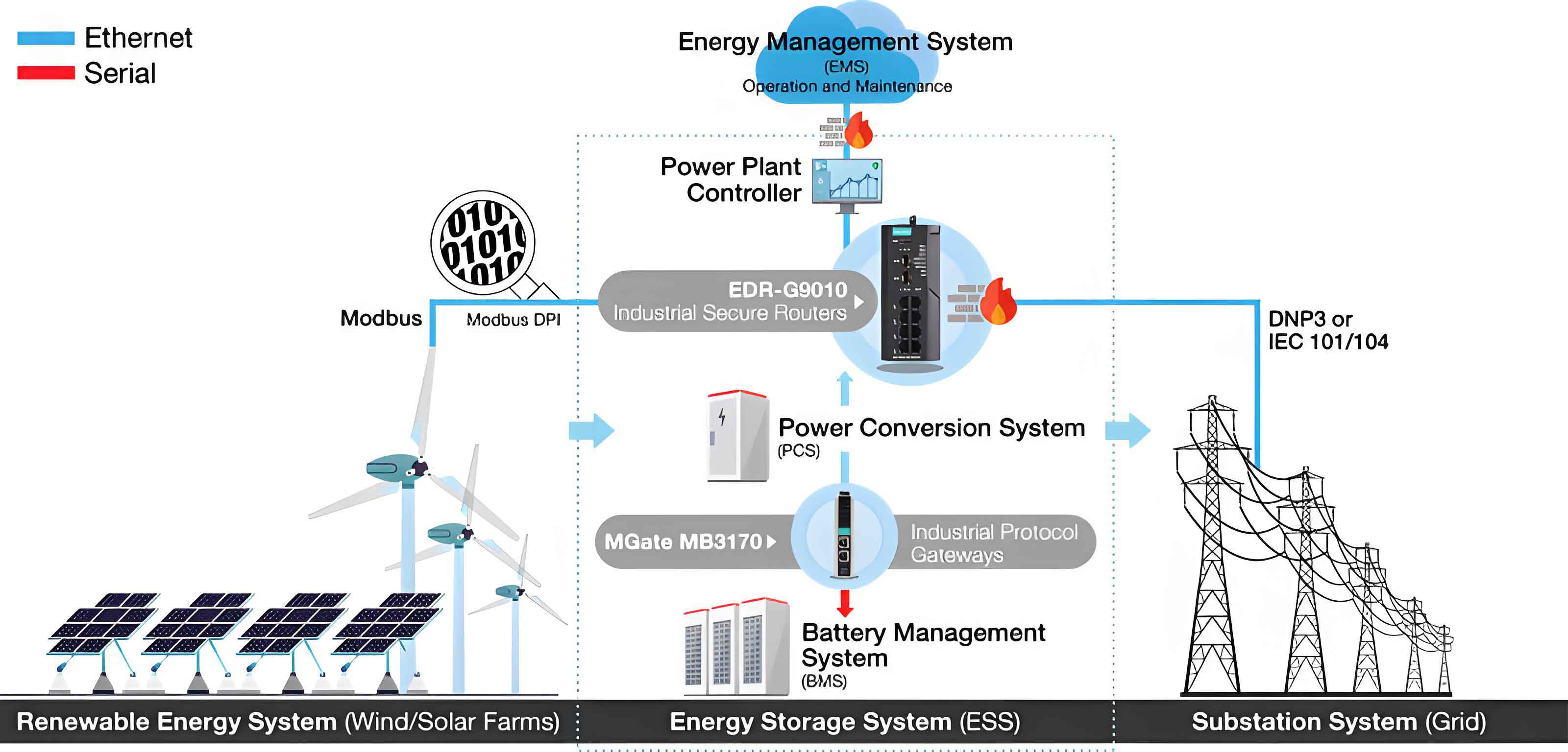
The proposed integrated energy system consists of an energy supply side, an energy conversion side, a hybrid energy storage side, and an energy consumption side. The energy supply side includes the external power grid, the natural gas network, and photovoltaic generation. The conversion side includes gas turbines, gas boilers, waste heat boilers, and electric boilers. The hybrid energy storage side includes compressed air energy storage, supercapacitors, and thermal energy storage. The consumption side includes electric load and thermal load. The system prioritizes photovoltaic power to satisfy the electric load. When photovoltaic power is insufficient, the system discharges the storage devices, activates gas turbines, or purchases electricity from the external grid. Surplus photovoltaic power can be stored in the compressed air energy storage or converted into thermal energy through the electric boiler. For the thermal load, the system primarily relies on gas turbines, gas boilers, electric boilers, and thermal energy storage. The coupling of various energy carriers and the flexible operation of the hybrid energy storage system enable the system to balance supply and demand effectively.
Energy Conversion Models
For the gas turbine, the electrical power output is expressed as a function of the consumed natural gas energy:
$$P_{GT}(t) = \eta_{GT} L_{NG} P_{GT}^{g}(t)$$
where \(P_{GT}(t)\) is the electrical output of the gas turbine at time \(t\), \(\eta_{GT}\) is the conversion efficiency, \(L_{NG}\) denotes the lower heating value of natural gas, and \(P_{GT}^{g}(t)\) is the natural gas input energy. The waste heat boiler recovers heat from the flue gas of the gas turbine as follows:
$$P_{HE}(t) = \frac{P_{GT}(t)}{\eta_{GT}} \eta_{HE}(1-\eta_{GT})$$
where \(\eta_{HE}\) is the waste heat boiler efficiency. The gas boiler model is given by:
$$Q_{GB}(t) = \eta_{GB} L_{NG} P_{GB}^{g}(t)$$
and the electric boiler model is:
$$Q_{EB}(t) = \eta_{EB} P_{EB}^{in}(t)$$
where \(Q_{GB}(t)\) and \(Q_{EB}(t)\) are the thermal outputs, \(\eta_{GB}\) and \(\eta_{EB}\) are the efficiencies, and \(P_{EB}^{in}(t)\) is the electrical input power of the electric boiler.
Hybrid Energy Storage Models
Compressed air energy storage operates in two modes. In the charging mode, the compression power is expressed as:
$$P_{Z,char} = \frac{m_A C_P T_{in}}{\eta_C} \left[ \left( \frac{P_{store}}{P_{atm}} \right)^{\frac{\gamma-1}{\gamma}} – 1 \right]$$
where \(m_A\) is the air mass flow rate, \(C_P\) is the specific heat capacity of air, \(T_{in}\) is the compressor inlet temperature, \(\eta_C\) is the compressor efficiency, \(P_{store}\) is the storage pressure, \(P_{atm}\) is the ambient pressure, and \(\gamma\) is the adiabatic index. The pressure dynamics inside the storage vessel are described by:
$$\frac{dP_{store}}{dt} = \frac{m_A R_A T_{store}}{M_A V_{store}}$$
In the discharging mode, the expansion power is given by:
$$P_{Z,dis} = m_A C_P T_{store} \left[ 1 – \left( \frac{P_{atm}}{P_{store}} \right)^{\frac{\gamma-1}{\gamma}} \right]$$
The supercapacitor model is simplified as an equivalent current-voltage formulation:
$$P_C = I_C V_C$$
where \(P_C\) is the charging or discharging power, \(I_C\) is the current, and \(V_C\) is the voltage. The thermal energy storage model is described by:
$$Q_S = m_S c_p \Delta T$$
where \(m_S\) is the mass of the storage medium, \(c_p\) is the specific heat capacity, and \(\Delta T\) is the temperature change.
Ultra-Short-Term Photovoltaic Interval Prediction
The accurate prediction of photovoltaic power plays a vital role in the optimal scheduling of an integrated energy system. Our interval prediction framework consists of four stages: data preprocessing, signal decomposition, component reconstruction, and interval prediction. The overall prediction process is illustrated in the following flowchart described in our earlier sections.
Data Preprocessing
To ensure the reliability and completeness of the raw photovoltaic power data, we first detect and remove outliers using the 3-sigma rule. For a normally distributed dataset, approximately 99.73% of the data points fall within the range \(\bar{x} \pm 3\sigma\). Any point outside this range is treated as an outlier. The missing values caused by outlier removal are then imputed using the k-nearest neighbors algorithm. The Mahalanobis distance is used to determine the nearest neighbors:
$$D(x) = \sqrt{(x-y)^T S^{-1} (x-y)}$$
where \(x\) is a single data point, \(y\) is the mean vector of the dataset, and \(S^{-1}\) is the inverse of the covariance matrix. After imputation, all data are normalized to the interval \([0,1]\) using min-max scaling:
$$x_1 = \frac{x_0 – x_{\min}}{x_{\max} – x_{\min}}$$
CEEMDAN-Based Signal Decomposition
The complete ensemble empirical mode decomposition with adaptive noise is applied to decompose the photovoltaic power series into multiple intrinsic mode functions. The algorithm adds adaptive white noise to the original signal to overcome modal mixing. The noise-added signal is generated as:
$$x_i(t) = x(t) + \beta_0 \varepsilon_i(t)$$
where \(\beta_0\) is the initial noise amplitude and \(\varepsilon_i(t)\) is the \(i\)-th Gaussian white noise. The first IMF is obtained by averaging the EMD results of the noise-added signals:
$$IMF_1(t) = \frac{1}{I} \sum_{i=1}^{I} EMD_1(x_i(t))$$
The first residual is:
$$r_1(t) = x(t) – IMF_1(t)$$
For later stages, the enhanced residual is:
$$r_k^{(i)}(t) = r_k(t) + \beta_k EMD_k(\varepsilon_i(t))$$
The decomposition continues until the residual becomes monotonic. The final reconstruction is:
$$x(t) = \sum_{k=1}^{K} IMF_k(t) + r_K(t)$$
Component Reconstruction with Permutation Entropy and PCA Clustering
After obtaining all IMFs, we calculate the permutation entropy of each IMF to evaluate its complexity. The permutation entropy is defined as:
$$H = -\sum_{i} p_i \log_2(p_i)$$
where \(p_i\) is the probability of the \(i\)-th ordinal pattern. Higher entropy indicates a more complex and random behavior. The permutation entropy values are then fed into a principal component analysis algorithm to reduce dimensionality and extract the main characteristics. The covariance matrix of the feature matrix \(H\) is given by:
$$C = \frac{1}{n-1} H H^T$$
After eigenvalue decomposition, the data matrix is projected onto the selected eigenvectors:
$$H_{pca} = H V_m$$
A K-means clustering algorithm is then applied to the projected features. The objective function of K-means clustering is:
$$E = \sum_{j=1}^{k} \sum_{h_i \in C_j} \left\| h_i – c_j \right\|^2$$
where \(c_j\) is the center of cluster \(C_j\). The IMFs are categorized into three components: a random component, a periodic component, and a trend component. This reconstruction reduces the non-stationarity of the original series and improves the prediction performance.
CQR-CNN-BiGRU Interval Prediction Model
Our interval prediction model combines conformalized quantile regression with a convolutional neural network and a bidirectional gated recurrent unit network. The convolutional neural network extracts hidden local features from the input time series. The one-dimensional convolution operation is expressed as:
$$(f \ast W)(x) = \sum_{i=0}^{k-1} f(x+i) \cdot W(i)$$
where \(W\) is the convolution kernel of size \(k\). The max-pooling layer reduces the feature dimension:
$$P_{\max}(f) = \max \{ f(x), f(x+1), \ldots, f(x+k-1) \}$$
The pooled features are then processed by a bidirectional gated recurrent unit network. The forward and backward hidden states are computed as:
$$h_t^{\rightarrow} = G(x_t, h_{t-1}^{\rightarrow})$$
$$h_t^{\leftarrow} = G(x_t, h_{t-1}^{\leftarrow})$$
The final hidden state is the weighted combination:
$$h_t = w_t h_t^{\rightarrow} + v_t h_t^{\leftarrow} + b_t$$
The convolutional neural network and the bidirectional gated recurrent unit network are jointly trained to predict the quantiles. The conformalized quantile regression method adjusts the prediction interval to guarantee a predefined coverage probability. The initial quantile regression generates a raw interval \([q_{low}(x), q_{up}(x)]\). Then, the conformity score is computed as:
$$E_i = \begin{cases} y_i – q_{up}(x_i), & y_i > q_{up}(x_i) \\ q_{low}(x_i) – y_i, & y_i < q_{low}(x_i) \\ 0, & \text{otherwise} \end{cases}$$
The final prediction interval is:
$$C(x) = [q_{low}(x) – Q_{1-\alpha}(E), \; q_{up}(x) + Q_{1-\alpha}(E)]$$
where \(Q_{1-\alpha}(E)\) is the \((1-\alpha)\)-quantile of the conformity scores. This approach gives an adaptive yet statistically valid interval.
Improved Sparrow Search Algorithm for Hyperparameter Optimization
To improve the prediction accuracy and interval quality, we use an improved sparrow search algorithm to optimize the hyperparameters of the convolutional neural network and the bidirectional gated recurrent unit network. The standard sparrow search algorithm suffers from low population diversity and easily falls into local optima. Therefore, we adopt three improvement strategies. First, we initialize the sparrow population using a reverse learning strategy:
$$Z_i’ = rand(L_b + U_b – Z_i)$$
where \(Z_i\) is an individual in the original population, \(Z_i’\) is its reverse individual, \(L_b\) and \(U_b\) are the lower and upper bounds of the parameter space. Second, we apply a dynamic step factor adjustment to control the step sizes \(\beta\) and \(k\):
$$\beta = \frac{f_b – f_w}{M – t} – f_b \cdot \frac{f_b – f_w}{M} \cdot t$$
$$k = (f_b – f_w) \cdot e^{\frac{-20 t}{M} \cdot \tan(rand(2\pi)) \cdot (2 rand – 1)}$$
where \(f_b\) is the best fitness, \(f_w\) is the worst fitness, \(M\) is the maximum iteration number, and \(t\) is the current iteration. Third, we introduce Levy flight to update the scout positions to avoid local optima:
$$z_{i,j}(t+1) = \begin{cases} z_{b,j}(t) + L(d) \cdot | z_{b,j}(t) – z_{w,j}(t) |, & f_i > f_b \\ z_{i,j}(t) + K \cdot \frac{z_{i,j}(t) – z_{g,j}(t)}{f_i – f_w + \epsilon}, & f_i = f_b \end{cases}$$
where \(L(d)\) is the Levy flight step length. The improved algorithm converges faster and finds better hyperparameters compared to the original sparrow search algorithm.
Evaluation Metrics for Interval Prediction
We use four standard metrics to evaluate the quality of the prediction intervals: the prediction interval coverage probability, the prediction interval normalized average width, the coverage width criterion, and the optimal confidence interval deviation. The prediction interval coverage probability is defined as:
$$PICP = \frac{1}{n} \sum_{i=1}^{n} c_i, \quad c_i = \begin{cases} 1, & y_i \in [L_i, U_i] \\ 0, & \text{otherwise} \end{cases}$$
The prediction interval normalized average width is:
$$PINAW = \frac{1}{nR} \sum_{i=1}^{n} (U_i – L_i)$$
where \(R\) is the range of the true values. The coverage width criterion is defined as:
$$CWC = PINAW \cdot (1 – PICP + e^{-\eta(1-\alpha)(1-PICP)})$$
where \(\eta\) is a penalty coefficient. Finally, the optimal confidence interval deviation is defined as:
$$D_{OCI} = \frac{|PICP – (1-\alpha)|}{1-\alpha} \times 100\%$$
In our experiments, the nominal confidence level \((1-\alpha)\) is set to 90%.
Prediction Results and Comparison
The proposed prediction model is tested on a public photovoltaic dataset with a 5-minute sampling resolution. The dataset covers one year of operation, and it is split into training, validation, and test sets. The data partitioning is shown in Table 1.
| Dataset | Time Range | Number of Samples |
|---|---|---|
| Training | 2015-09-21 to 2016-04-29 | 63,360 |
| Validation | 2016-04-29 to 2016-07-11 | 21,024 |
| Test | 2016-07-11 to 2016-09-21 | 21,024 |
The CEEMDAN method decomposes the original series into twelve IMFs and one residual component. The permutation entropy values of these IMFs are listed in Table 2.
| IMF | IMF1 | IMF2 | IMF3 | IMF4 | IMF5 | IMF6 |
|---|---|---|---|---|---|---|
| PE | 0.16574 | 0.29728 | 0.52876 | 0.76025 | 0.67329 | 0.31263 |
| IMF | IMF7 | IMF8 | IMF9 | IMF10 | IMF11 | IMF12 |
|---|---|---|---|---|---|---|
| PE | 0.26945 | 0.10467 | 0.04651 | 0.04382 | 0.02137 | 0.00368 |
Applying the principal component analysis clustering yields three component groups as shown in Table 3.
| Component Type | IMFs |
|---|---|
| Random component | IMF3, IMF4, IMF5 |
| Periodic component | IMF1, IMF2, IMF6, IMF7 |
| Trend component | IMF8, IMF9, IMF10, IMF11, IMF12 |
We compare the proposed model with four benchmark models: QR-GRU, QR-BiGRU, CQR-CNN-BiGRU, and CEEMDAN-CNN-BiGRU. All models are optimized with the improved sparrow search algorithm where applicable. The interval prediction performance at the 90% confidence level is summarized in Table 4.
| Model | PICP | PINAW | CWC | Optimal Confidence Deviation |
|---|---|---|---|---|
| QR-GRU | 96.8% | 0.185 | 0.778 | 6.8% |
| QR-BiGRU | 96.9% | 0.147 | 0.813 | 6.9% |
| CQR-CNN-BiGRU | 93.4% | 0.139 | 0.852 | 3.4% |
| CEEMDAN-CNN-BiGRU | 92.4% | 0.126 | 0.869 | 2.4% |
| Proposed model | 91.1% | 0.115 | 0.883 | 1.1% |
It can be observed that all models satisfy the nominal coverage requirement of 90%. However, the proposed model achieves the closest PICP to the ideal value of 90%, with a deviation of only 1.1%. The PINAW of the proposed model is 0.115, which is much narrower than those of the benchmark models. This indicates that the proposed interval prediction model provides more informative and reliable prediction intervals. The high CWC value also confirms the overall superiority of the proposed method.
Bi-Level Optimization Configuration of Hybrid Energy Storage System
Based on the photovoltaic interval prediction results, we formulate a bi-level optimization framework for the capacity configuration and operation scheduling of the integrated energy system. The upper level determines the capacities of the compressed air energy storage and supercapacitor energy storage with the objective of minimizing the total life-cycle cost of the hybrid energy storage system. The lower level optimizes the day-ahead dispatch of all energy devices with the objective of minimizing the total operating cost of the integrated energy system. The upper-level capacity results act as boundary constraints for the lower-level optimization, while the lower-level operational results are fed back to the upper level to verify the feasibility of the capacity configuration. The iterative process continues until convergence.
Upper-Level Model
The objective function of the upper-level model minimizes the total cost of the hybrid energy storage system, including the investment cost and the operation and maintenance cost:
$$\min \; C_1 = C_C^i + C_Z^i + C_C^p + C_Z^p$$
The investment cost of the supercapacitor energy storage is:
$$C_C^i = \frac{\alpha_c (1+\alpha_c)^{T_c}}{(1+\alpha_c)^{T_c} – 1} \left( k_{C,P} P_C + k_{C,E} E_C \right)$$
where \(P_C\) and \(E_C\) are the rated power and capacity of the supercapacitor, \(k_{C,P}\) and \(k_{C,E}\) are the unit power cost and unit capacity cost, \(\alpha_c\) is the discount rate, and \(T_c\) is the lifetime. Similarly, the investment cost of the compressed air energy storage is:
$$C_Z^i = \frac{\alpha_z (1+\alpha_z)^{T_z}}{(1+\alpha_z)^{T_z} – 1} \left( k_{Z,P} P_Z + k_{Z,E} E_Z \right)$$
The operation and maintenance costs are proportional to the investment costs:
$$C_C^p = a_C C_C^i, \quad C_Z^p = a_Z C_Z^i$$
where \(a_C\) and \(a_Z\) are the operation and maintenance cost coefficients.
The upper-level constraints include the charging and discharging power limits:
$$-P_C^n \leq P_C(t) \leq P_C^n$$
$$-P_Z^n \leq P_Z(t) \leq P_Z^n$$
and the state-of-charge constraints:
$$SOC_{C,\min} \leq SOC_C(t) \leq SOC_{C,\max}$$
$$SOC_{Z,\min} \leq SOC_Z(t) \leq SOC_{Z,\max}$$
Lower-Level Model
The lower-level model minimizes the total day-ahead operating cost of the integrated energy system, which consists of the electricity purchase and sale cost, the gas purchase cost, the equipment operation and maintenance cost, and the reliability cost:
$$\min \; C_2 = C_e + C_g + C_{om} + C_k$$
The electricity purchase and sale cost is:
$$C_e = \sum_{t=1}^{T} \left[ P_{buy}(t) \cdot \pi_{buy}(t) – P_{sell}(t) \cdot \pi_{sell}(t) \right]$$
where \(P_{buy}(t)\) and \(P_{sell}(t)\) are the purchased and sold electricity powers, and \(\pi_{buy}(t)\) and \(\pi_{sell}(t)\) are the corresponding time-of-use prices. The gas purchase cost is:
$$C_g = \pi_{gas}(t) \sum_{t=1}^{T} \left[ \frac{P_{GT}(t)}{L_{NG}} + \frac{P_{GB}(t)}{L_{NG}} \right]$$
The operation and maintenance cost is:
$$C_{om} = \sum_{t=1}^{T} \left[ c_{GT} P_{GT}(t) + c_{GB} P_{GB}(t) + c_{EB} Q_{EB}(t) + c_{HE} P_{HE}(t) + c_R P_R(t) \right]$$
The reliability cost accounts for load shedding and curtailed photovoltaic power:
$$C_k = \sum_{t=1}^{T} W(t)$$
where \(W(t)\) is the weighted sum of lost electric load, lost thermal load, and curtailed photovoltaic power at time \(t\).
The lower-level constraints include the electric power balance:
$$P_{PV}(t) + P_{GT}(t) + P_C(t) + P_Z(t) + P_{EB}^{in}(t) + P_{buy}(t) = P_L(t) + P_{EB}^{out}(t) + P_{sell}(t) + P_{PV}^{curt}(t) + P_{load}^{sh}(t)$$
and the thermal power balance:
$$Q_{GT}(t) + Q_{GB}(t) + Q_{EB}(t) + Q_{S,dis}(t) + Q_{Z,out}(t) = Q_L(t) + Q_{S,char}(t) + Q_{Z,in}(t) + Q_{load}^{sh}(t)$$
The device output constraints are given by:
$$Q_{i,\min} \leq Q_i(t) \leq Q_{i,\max}, \quad i \in \{GT, GB, EB\}$$
The external network transmission constraints are:
$$0 \leq P_{buy}(t) \leq w(t) P_{buy}^{\max}$$
$$0 \leq P_{sell}(t) \leq (1-w(t)) P_{sell}^{\max}$$
where \(w(t)\) is a binary variable indicating the purchase or sale state. The thermal storage constraints are:
$$0 \leq Q_{S,dis}(t) \leq n(t) Q_{S,dis}^{\max}$$
$$0 \leq Q_{S,char}(t) \leq (1-n(t)) Q_{S,char}^{\max}$$
$$Q_{S,\min} \leq Q_S(t) \leq Q_{S,\max}$$
Demand Response Modeling
To further improve the economic performance and the load profile, we introduce a price-based demand response program. The total load before and after demand response remains unchanged:
$$\sum_{t=1}^{T} \Delta q_t = 0$$
The price elasticity of demand links the load change ratio and the price change ratio:
$$\frac{\Delta q_t}{q_t} = \varepsilon \frac{\Delta p_t}{p_t}$$
where \(\varepsilon\) is the elasticity coefficient. The load is divided into peak, flat, and valley periods, and the cross-elasticity matrix is constructed as:
$$\begin{bmatrix} \Delta q_f / q_f \\ \Delta q_p / q_p \\ \Delta q_g / q_g \end{bmatrix} = \begin{bmatrix} \varepsilon_{ff} & \varepsilon_{fp} & \varepsilon_{fg} \\ \varepsilon_{pf} & \varepsilon_{pp} & \varepsilon_{pg} \\ \varepsilon_{gf} & \varepsilon_{gp} & \varepsilon_{gg} \end{bmatrix} \begin{bmatrix} \Delta p_f / p_f \\ \Delta p_p / p_p \\ \Delta p_g / p_g \end{bmatrix}$$
After demand response, the electric and thermal load curves become smoother, which reduces the peak-to-valley difference and eases the pressure on the energy storage system.
Case Study and Discussions
We set up three comparison scenarios to evaluate the proposed method. Scenario 1 considers only electric hybrid energy storage without thermal energy storage. Scenario 2 considers both electric and thermal hybrid energy storage. Scenario 3 incorporates the ultra-short-term photovoltaic interval prediction proposed in this work together with electric and thermal hybrid energy storage. The system parameters are summarized in Table 5.
| Parameter | Value |
|---|---|
| Gas turbine O&M coefficient | 0.1685 |
| Gas boiler O&M coefficient | 0.0018 |
| Electric boiler O&M coefficient | 0.0125 |
| Waste heat boiler O&M coefficient | 0.0065 |
| Gas turbine max output | 1000 kW |
| Gas boiler max output | 1000 kW |
| Electric boiler max output | 500 kW |
| Gas turbine electrical efficiency | 0.35 |
| Gas turbine thermal efficiency | 0.85 |
| Gas boiler efficiency | 0.90 |
| Electric boiler efficiency | 0.93 |
| Waste heat boiler efficiency | 0.90 |
| Thermal storage capacity upper limit | 1800 kWh |
The time-of-use electricity and gas prices are shown in Table 6 and Table 7, respectively.
| Period | Time slots | Purchase price (CNY/kWh) |
|---|---|---|
| Peak | 8:00-12:00, 19:00-22:00 | 1.21 |
| Flat | 13:00-18:00 | 0.73 |
| Valley | 1:00-7:00, 23:00-24:00 | 0.45 |
| Period | Time slots | Gas price (CNY/m³) |
|---|---|---|
| Peak | 1:00-6:00, 13:00-18:00, 23:00-24:00 | 2.05 |
| Valley | 7:00-12:00, 19:00-22:00 | 1.57 |
The optimal capacities of the hybrid energy storage system in the three scenarios are shown in Table 8.
| Scenario | Compressed air storage (kWh) | Supercapacitor (kWh) | Thermal storage (kWh) |
|---|---|---|---|
| Scenario 1 | 1651.44 | 986.31 | 0 |
| Scenario 2 | 3533.13 | 572.20 | 1465.09 |
| Scenario 3 | 4074.96 | 890.91 | 1904.30 |
The daily operating costs of the integrated energy system for the three scenarios are compared in Table 9.
| Scenario | Total operating cost (CNY) | Electricity selling revenue (CNY) | Electricity purchase cost (CNY) | Gas purchase cost (CNY) | O&M cost (CNY) | Reliability cost (CNY) |
|---|---|---|---|---|---|---|
| Scenario 1 | 58439.92 | 0 | 17560.31 | 30066.41 | 1966.10 | 8847.10 |
| Scenario 2 | 50405.64 | 371.97 | 13665.36 | 27398.73 | 2084.50 | 7629.02 |
| Scenario 3 | 47261.58 | 548.50 | 12723.46 | 26896.12 | 2016.52 | 6173.98 |
The comparison between Scenario 1 and Scenario 2 shows that the addition of thermal energy storage reduces the total operating cost by 13.75%. The electricity purchase cost decreases by 22.18%, the gas purchase cost decreases by 8.87%, and the reliability cost decreases by 13.77%. The electricity selling revenue also increases to 371.97 CNY. This improvement is mainly due to the ability of thermal energy storage to decouple the combined heat and power constraint, which enhances the operational flexibility of the gas turbine and compressed air energy storage.
The comparison between Scenario 2 and Scenario 3 shows that incorporating photovoltaic interval prediction further reduces the total operating cost by 6.24%. The electricity purchase cost decreases by 6.89%, the gas purchase cost decreases by 1.83%, and the reliability cost decreases by 19.07%. The electricity selling revenue increases by 47.46%. The improvement arises from the more accurate prediction of photovoltaic power, which allows the storage capacity to be allocated more precisely according to the random and periodic components of the photovoltaic power series. Consequently, the system curtails less photovoltaic power, sheds fewer loads, and operates more economically.
The electric power balance of Scenario 3 is analyzed as follows. During the valley price period from 22:00 to 08:00, the system purchases cheap electricity from the grid. Part of this electricity is used to meet the electric load, and the surplus is stored in the compressed air energy storage. Some electricity is also converted into thermal energy through the electric boiler to meet the thermal load. During the daytime from 09:00 to 15:00, photovoltaic power becomes abundant and is preferentially used to meet the electric load. Supercapacitors smooth the short-term fluctuations of photovoltaic power. During the evening peak period, the compressed air energy storage discharges to supplement the gas turbine output, ensuring a reliable supply of electricity. The thermal power balance shows that during the night valley period, the electric boiler and gas boiler jointly supply heat. During the daytime and evening, the gas turbine and gas boiler are the main heat sources, while the thermal energy storage absorbs and releases heat to accommodate the varying operational states of the gas turbine and compressed air energy storage.
The demand response analysis is presented in Table 10. After implementing the price-based demand response, the peak-to-valley difference of the electric load decreases from 1290 kW to 960 kW, a reduction of 25.58%. The peak-to-valley difference of the thermal load decreases from 596 kW to 578.4 kW, a reduction of only 2.95%. This indicates that demand response has a significant effect on shifting electric load and smoothing the electric load profile. The effect on thermal load is less obvious because users are less sensitive to small temperature variations in heat supply.
| Load type | Before DR (kW) | After DR (kW) | Reduction |
|---|---|---|---|
| Electric load | 1290 | 960 | 25.58% |
| Thermal load | 596 | 578.4 | 2.95% |
Conclusion and Future Work
In this work, we proposed a hybrid energy storage system optimization method for an integrated energy system based on ultra-short-term photovoltaic interval prediction. We established a bi-level optimization model that coordinates the capacity configuration of the hybrid energy storage system in the upper level and the operational scheduling of the integrated energy system in the lower level. The upper level uses the photovoltaic interval prediction results, especially the decomposition into random, periodic and trend components, to establish the capacity boundary of the compressed air energy storage and supercapacitor energy storage. The lower level then optimizes the day-ahead dispatch with the objective of minimizing the total operating cost while satisfying all operational constraints.
The experimental results demonstrate the effectiveness of the proposed photovoltaic interval prediction model. The proposed CEEMDAN-PE-PCA-CQR-CNN-BiGRU model achieves a prediction interval coverage probability of 91.1%, a prediction interval normalized average width of 0.115, and an optimal confidence interval deviation of only 1.1%. The narrower interval width and the higher coverage width criterion indicate that the model provides both reliable and sharp prediction intervals.
The case study of the integrated energy system shows that the incorporation of thermal energy storage significantly improves the economic and operational flexibility of the system. The total operating cost is reduced by 13.75% when thermal energy storage is added. The use of photovoltaic interval prediction further reduces the total operating cost by 6.24% and reduces the reliability cost by 19.07%, which means less load shedding and less photovoltaic curtailment. Demand response also plays a positive role in flattening the load profile, especially for the electric load.
In future research, we will extend the proposed approach to consider the uncertainty of both supply and demand sides. The current work focuses mainly on the uncertainty of photovoltaic power, while the load side also exhibits stochastic characteristics. A comprehensive uncertainty quantification model that considers both renewable generation and load demand would further improve the operational reliability. Moreover, the proposed interval prediction framework can be extended to other renewable energy sources, such as wind power, to create a more general uncertainty forecasting tool. In addition, the dynamic characteristics of different energy storage devices and energy conversion equipment should be more precisely modeled to enhance the applicability of the proposed method in practical engineering.