
In this article I present a composite control strategy for single-phase grid-connected solar inverters. The proposed method combines an embedded repetitive controller with state-feedback current control, and it adds both DC-voltage feed-forward decoupling and grid-voltage feed-forward compensation. This architecture is designed to eliminate the filter resonant peak, to suppress low-order harmonic disturbances caused by DC-link pulsation, grid distortion, and switch dead-time, and to give the grid-connected inverter zero steady-state tracking error with fast dynamic response. I explain the system model, harmonic characteristics, control design, stability condition, and experimental verification of the method. Throughout the article I emphasize practical issues that arise in modern solar inverters.
Abstract
Grid-connected solar inverters must inject high-quality currents into the grid. An LCL filter is often preferred because it provides better high-frequency attenuation than a single inductor. However, the LCL filter introduces a resonance peak that can make the current loop unstable. In addition, low-order harmonics are generated by the DC-link voltage ripple, dead-time effects, and grid voltage distortion. I propose a composite current controller in which state feedback performs pole placement, a repetitive controller provides periodic harmonic compensation, DC-voltage feed-forward stabilizes the inverter gain, and grid-voltage feed-forward cancels the mains disturbance. The resulting control system has high robustness, fast transient response, and very low steady-state current distortion.
Introduction
The increasing penetration of distributed photovoltaic generation has made the power quality of solar inverters an important topic. Grid standards impose strict limits on the harmonic content of the injected current. A simple L filter may require a large inductance in order to attenuate switching harmonics, but this increases size, cost, and losses. The LCL filter is a common alternative because its third-order attenuation characteristic allows smaller magnetic components. Nevertheless, the LCL network has a resonant frequency at which the plant gain becomes very high. Without extra damping, this resonance can amplify current harmonics and cause instability.
Traditional PI regulators are widely used in current-controlled solar inverters. They are simple to implement, but they have finite gain at the fundamental frequency and cannot completely reject periodic disturbances. The internal model principle states that a disturbance can be rejected with zero steady-state error only if the controller contains a model of the disturbance. For periodic disturbances such as dead-time harmonics and grid harmonics, the repetitive controller provides such a model. A repetitive controller includes a delay line of one fundamental period and can produce very large gain at multiples of the fundamental frequency. However, the period delay in a purely repetitive controller slows the transient response. I therefore use an embedded or plug-in repetitive controller that keeps the fast reference path intact while the repetitive loop compensates only the periodic error.
The strategy described here is specifically designed for solar inverters that must operate in a weak grid where the grid voltage is distorted and the DC bus is not perfectly constant. I first derive the LCL plant model and analyze the harmonic sources. Then I design a state-feedback controller by pole placement to damp the resonance. I add a DC-voltage feed-forward path to make the average inverter bridge gain independent of the actual DC-link voltage. I also add a grid-voltage feed-forward path to reject the grid voltage disturbance. Finally, I embed a repetitive controller around the closed-loop system to handle periodic low-order harmonics. The combination gives excellent performance for modern solar inverters.
System Model and Harmonic Characteristics
The power stage considered here is a single-phase full-bridge inverter connected to the grid through an LCL filter. The DC side is supplied by a photovoltaic array through a DC-DC converter. The inverter bridge produces a pulse-width-modulated voltage, and the LCL filter converts this voltage into a smooth grid current. The symbols used throughout the article are summarized below.
| Symbol | Meaning |
| Udc | DC-link voltage |
| Cdc | DC-link capacitance |
| L1, R1 | Inverter-side inductor and its parasitic resistance |
| Cf | LCL filter capacitance |
| L2, R2 | Grid-side inductor and its parasitic resistance |
| i1 | Inverter-side inductor current |
| vC | Voltage across the filter capacitor |
| ig = i2 | Grid current |
| vg | Grid voltage at the point of common coupling |
| vinv | Average inverter bridge output voltage |
| d | Duty-cycle signal produced by the PWM modulator |
| fs | Switching and sampling frequency |
| f0 | Grid fundamental frequency |
| N | Number of sampling periods in one fundamental period |
Using Kirchhoff’s laws for the LCL filter, the dynamic equations are
$$
\begin{aligned}
\frac{\mathrm{d}i_1}{\mathrm{d}t} &= \frac{1}{L_1}\left(v_{\mathrm{inv}} – v_C – R_1 i_1\right) \\
\frac{\mathrm{d}v_C}{\mathrm{d}t} &= \frac{1}{C_f}\left(i_1 – i_2\right) \\
\frac{\mathrm{d}i_2}{\mathrm{d}t} &= \frac{1}{L_2}\left(v_C – v_g – R_2 i_2\right)
\end{aligned}
$$
In state-space form, with \(\boldsymbol{x} = [i_1, v_C, i_2]^T\), the plant becomes
$$
\frac{\mathrm{d}}{\mathrm{d}t}
\begin{bmatrix}
i_1 \\
v_C \\
i_2
\end{bmatrix}
=
\begin{bmatrix}
-\frac{R_1}{L_1} & -\frac{1}{L_1} & 0 \\
\frac{1}{C_f} & 0 & -\frac{1}{C_f} \\
0 & \frac{1}{L_2} & -\frac{R_2}{L_2}
\end{bmatrix}
\begin{bmatrix}
i_1 \\
v_C \\
i_2
\end{bmatrix}
+
\begin{bmatrix}
\frac{1}{L_1} \\
0 \\
0
\end{bmatrix}
v_{\mathrm{inv}}
+
\begin{bmatrix}
0 \\
0 \\
-\frac{1}{L_2}
\end{bmatrix}
v_g
$$
The transfer function from the inverter bridge voltage to the grid current is
$$
P(s)=\frac{I_2(s)}{V_{\mathrm{inv}}(s)}
=
\frac{1}{L_1L_2C_f s^3 + (L_1R_2+L_2R_1)C_f s^2 + (L_1+L_2+R_1R_2C_f)s + R_1+R_2}
$$
Neglecting the parasitic resistances for the purpose of resonance analysis gives
$$
P(s) \approx \frac{1}{L_1L_2C_f s\left(s^2+\omega_{\mathrm{res}}^2\right)}
$$
$$
\omega_{\mathrm{res}} = \sqrt{\frac{L_1+L_2}{L_1L_2C_f}}
$$
The LCL resonance appears as a high peak in the frequency response. This peak is a well-known challenge for current control of grid-connected solar inverters. Without damping, the gain at the resonant frequency is very high and may amplify grid background distortion and switching sidebands.
The inverter bridge itself can be represented by an average model
$$
v_{\mathrm{inv}}(t)=d(t)\,U_{\mathrm{dc}}(t)
$$
In a unipolar sine pulse-width modulator, the switching frequency of the output voltage ripple is twice the carrier frequency. A double Fourier series for the bridge output voltage can be written as
$$
v_{\mathrm{inv}}(t)=U_{\mathrm{dc}}
\left[
M\cos(\omega_0 t)
+
\sum_{m=1}^{\infty}
\sum_{n=-\infty}^{\infty}
A_{mn}
\cos(m\omega_c t + n\omega_0 t)
\right]
$$
where \(M\) is the modulation index, \(\omega_0\) is the grid angular frequency, \(\omega_c\) is the carrier angular frequency, and \(A_{mn}\) are Bessel-function coefficients. The high-order switching sidebands are easily attenuated by the LCL filter. The main problem is caused by low-order harmonics near the fundamental frequency, because an LCL filter cannot remove them without impractically large reactive components.
For solar inverters, the important harmonic sources are the DC-link voltage ripple, the grid voltage distortion, and the dead-time effect. The DC-link voltage of single-phase photovoltaic inverters always contains a second-order ripple at twice the grid frequency. This ripple can be expressed as
$$
U_{\mathrm{dc}}(t)=U_{\mathrm{dc}0} + U_{\mathrm{dc}2}\cos(2\omega_0 t+\varphi_2)
$$
When this ripple is multiplied by the modulating signal, sidebands appear around the fundamental component. These sidebands are asymmetric and give rise to odd current harmonics. In addition, dead-time causes an error voltage that is nearly a square wave in phase with the grid current. The average dead-time error can be approximated by
$$
v_{\mathrm{err}}(t) \approx \frac{t_d U_{\mathrm{dc}}}{T_s}\,\mathrm{sign}\left(i_g(t)\right)
$$
This square-wave-like voltage contains strong third, fifth, seventh, and other odd harmonics. Finally, a weak grid may contain significant low-order harmonics in the grid voltage, and these harmonics produce corresponding currents because the output impedance of the inverter is finite. The main harmonic sources and their effects are summarized in the following table.
| Disturbance source | Harmonic effect | Preferred countermeasure |
| DC-link 2nd-order voltage ripple | Odd current harmonics through cross-modulation | DC-voltage feed-forward decoupling |
| Grid voltage distortion | 3rd, 5th, 7th current harmonics | Grid-voltage feed-forward and repetitive control |
| Dead-time effect | Low-order odd harmonics | Repetitive control, dead-time compensation |
| LCL resonance | Oscillation near resonance frequency | State-feedback pole placement |
Composite Control Architecture
The architecture that I propose uses four parallel elements in the current loop.
The first element is a state-feedback controller that places the closed-loop poles of the LCL plant at desired positions. This eliminates the resonance peak and provides a well-damped plant for the outer controllers. The second element is a reference feed-forward gain that gives the inner closed-loop system unity DC gain. The third element is a repetitive controller that is embedded in a plug-in configuration. The repetitive controller operates on the current error and produces a correction signal only when the error contains periodic components. The fourth element is a combination of two feed-forward paths: one from the DC-link voltage and one from the grid voltage.
The total normalized duty command can be written as
$$
d=\frac{v_{\mathrm{ctrl}}}{U_{\mathrm{dc}}}
$$
where \(v_{\mathrm{ctrl}}\) is the desired bridge voltage generated by the controller. This normalization is important because the actual bridge output voltage is the product of the duty cycle and the DC-link voltage. By dividing by the measured \(U_{\mathrm{dc}}\), I make the average bridge gain independent of DC-link voltage changes.
The desired bridge voltage is composed of state feedback, reference feed-forward, repetitive correction, and grid-voltage feed-forward:
$$
v_{\mathrm{ctrl}} = – \boldsymbol{K}\boldsymbol{x} + k_r i^* + u_{\mathrm{rep}} + K_g \hat{v}_g
$$
where \(\boldsymbol{K}\) is the state-feedback gain matrix, \(k_r\) is the reference feed-forward gain, \(u_{\mathrm{rep}}\) is the output of the repetitive controller, \(\hat{v}_g\) is the measured grid voltage, and \(K_g\) is the grid feed-forward coefficient. In the simplest practical implementation I use \(K_g=1\), which is a partial feed-forward that is very effective at low frequencies.
State-Feedback Pole Placement
The open-loop LCL plant is a third-order system. With small parasitic resistances, the open-loop poles are located close to the imaginary axis. The natural dynamic response is therefore poorly damped. State feedback can be used to move all three poles to desired locations.
Let the desired characteristic polynomial be
$$
P_d(s)=(s^2+2\zeta\omega_n s+\omega_n^2)(s+p_3)
$$
where \(\zeta\) is the desired damping ratio, \(\omega_n\) is the desired natural frequency, and \(p_3\) is the third pole. In my design I chose
$$
\zeta=0.8
$$
$$
\omega_n=3000\ \mathrm{rad/s}
$$
$$
p_3=12000\ \mathrm{rad/s}
$$
so that the desired closed-loop poles are
$$
p_{1,2}=-2400 \pm j1800
$$
$$
p_3=-12000
$$
The third pole is placed far to the left in the complex plane. It therefore has little influence on the dominant response. The closed-loop characteristic polynomial is
$$
(s^2+4800s+9\times10^6)(s+12000)
=
s^3+16800s^2+57.6\times10^6s+108\times10^9
$$
Using the controllability matrix
$$
\mathcal{C}=
\begin{bmatrix}
\boldsymbol{B} & \boldsymbol{A}\boldsymbol{B} & \boldsymbol{A}^2\boldsymbol{B}
\end{bmatrix}
$$
the state-feedback gain vector \(\boldsymbol{K}\) can be calculated by the Ackermann formula
$$
\boldsymbol{K}
=
\begin{bmatrix}
0 & 0 & 1
\end{bmatrix}
\mathcal{C}^{-1}
P_d(\boldsymbol{A})
$$
where \(P_d(\boldsymbol{A})\) is the matrix version of the desired polynomial. This calculation gives a direct expression for the state-feedback gains in terms of the LCL parameters.
After state feedback, the closed-loop system from the auxiliary control input to the grid current has the transfer function
$$
P_{sc}(s)=
\frac{P(s)}{1+\boldsymbol{K}\Phi(s)\boldsymbol{B}}
$$
Where \(\Phi(s)=(s\boldsymbol{I}-\boldsymbol{A})^{-1}\). The resonance peak is effectively eliminated because the conjugate pair is moved away from the imaginary axis.
The reference feed-forward gain \(k_r\) is selected so that the closed-loop DC gain from the current reference \(i^*\) to the grid current is unity. The formula is
$$
k_r=-\left[\boldsymbol{C}\left(\boldsymbol{A}-\boldsymbol{B}\boldsymbol{K}\right)^{-1}\boldsymbol{B}\right]^{-1}
$$
With this gain, a step in the current reference is tracked without steady-state error for a nominal plant. The state-feedback loop therefore provides fast and well-damped tracking for the fundamental component.
In the practical implementation, all three states of the LCL filter are not always measured directly. The input-side current \(i_1\) and grid current \(i_2\) can be obtained from current sensors, while the capacitor voltage \(v_C\) can be reconstructed with a Luenberger observer. The separation principle guarantees that the observer poles do not need to be coupled with the controller poles. I used observer poles approximately three times faster than the dominant closed-loop poles so that the observer does not disturb the desired dynamic response.
DC-Voltage and Grid-Voltage Feed-Forward
Single-phase solar inverters often have a DC-link voltage that contains a strong ripple at twice the grid frequency. This ripple is caused by instantaneous power imbalance between the DC input and the AC output. If the modulation controller ignores the DC ripple, the bridge output voltage contains low-order harmonics propagated from the DC side.
My solution is a direct algebraic feed-forward. The PWM modulator receives a duty command
$$
d=\frac{v_{\mathrm{ctrl}}}{U_{\mathrm{dc}}}
$$
When \(U_{\mathrm{dc}}\) increases, the duty-cycle is reduced automatically; when \(U_{\mathrm{dc}}\) decreases, the duty-cycle increases. This makes the average bridge output voltage equal to \(v_{\mathrm{ctrl}}\) regardless of DC-link changes. The DC-voltage feed-forward decouples the current control loop from the DC-link dynamics.
The grid voltage is another disturbance input. Full rejection of the grid voltage would require a feed-forward transfer function equal to
$$
K_{g,\mathrm{full}}(s)=1+sR_1C_f+s^2L_1C_f
$$
This expression contains a second-order derivative term \(s^2L_1C_f\), which strongly amplifies measurement noise. In practice the second-order term is negligible in the low-frequency range where the harmonic compensation is needed. For the fundamental frequency of 50 Hz, the term \(s^2L_1C_f\) has a magnitude of only about 0.1% for the parameters used in my prototype. Even at the fifth harmonic it is still very small. I therefore use the partial feed-forward \(K_g=1\)
$$
u_{\mathrm{ff},g}=\hat{v}_g
$$
This simple feed-forward path ensures that the inverter bridge reproduces the grid voltage component at the output, thereby reducing the voltage difference across the grid-side inductor and suppressing current harmonics caused by the grid background voltage. It is much easier to implement than the full second-order feed-forward because no derivative filtering is required.
Repetitive Controller Design for Periodic Harmonics
State feedback and the two feed-forward paths are not sufficient to remove all low-order harmonics. Dead-time harmonics, grid harmonics, and DC-link effects may still produce periodic current errors. To reject these periodic disturbances, I use a repetitive controller. The internal model of a periodic signal with fundamental period \(T_0\) is
$$
G_{\mathrm{RM}}(z)=\frac{Q(z)z^{-N}}{1-Q(z)z^{-N}}
$$
where \(N\) is the number of samples per fundamental period,
$$
N=\frac{f_s}{f_0}
$$
and \(Q(z)\) is a low-pass filter or a constant close to unity. For my experimental system, \(f_s=20\ \mathrm{kHz}\) and \(f_0=50\ \mathrm{Hz}\), so \(N=400\). The complete repetitive controller is
$$
G_{rp}(z)=\frac{Q(z)z^{-N}}{1-Q(z)z^{-N}}
\,
k_{rp}
\,
C(z)
$$
Here \(k_{rp}\) is the repetitive control gain and \(C(z)\) is a phase compensator. The phase compensator is selected as
$$
C(z)=z^m S(z)
$$
where \(m\) is the number of leading steps used to compensate for the delay of the controlled plant, and \(S(z)\) is a low-pass filter that increases high-frequency attenuation. In my implementation I used
$$
Q(z)=0.98
$$
$$
k_{rp}=0.85
$$
$$
S(z)=\frac{1-\alpha}{1-\alpha z^{-1}}
$$
$$
\alpha=0.8
$$
The repetitive controller output is added to the desired bridge voltage
$$
u_{\mathrm{rep}}(z)=G_{rp}(z)e(z)
$$
where \(e(z)=i^*(z)-i_g(z)\). Because the repetitive controller is embedded in parallel with the state-feedback path, the reference current does not have to wait for the repetitive delay. The fast dynamic path remains direct from \(i^*\) to the modulation signal.
The error transfer function of the outer loop can be written as
$$
E(z)=\frac{R(z)-D(z)}{1+P_{sc}(z)G_{rp}(z)}
$$
Where \(P_{sc}(z)\) is the closed-loop plant after state feedback. A sufficient stability condition for the combined system is
$$
\left\|
Q(e^{j\omega T})
\left[
1 – k_{rp}C(e^{j\omega T})P_{sc}(e^{j\omega T})
\right]
\right\|_{\infty}
< 1
$$
This condition means that the phase compensator \(C(z)\) must make the compensated plant \(C(z)P_{sc}(z)\) close to unity in the low-frequency and mid-frequency range. At harmonic frequencies where \(z^{-N}=1\), the open-loop gain of the repetitive controller becomes very large. Therefore periodic disturbances are attenuated by a large factor and the steady-state current error approaches zero in the ideal case \(Q=1\). In practice \(Q=0.98\) is used to improve robustness without significantly increasing harmonic error.
The important advantage of the embedded repetitive controller can be seen by comparing two structures. In a series repetitive controller, the entire reference signal passes through the \(z^{-N}\) delay. This forces the grid current to wait one fundamental cycle before responding to a reference change. In the embedded structure, the repetitive controller is only one of several parallel branches. The reference tracking path does not contain the repetitive delay. The correction path still contains the \(z^{-N}\) memory, but it acts only on the error signal. This improves the transient behavior of the solar inverters without sacrificing harmonic rejection.
| Block | Design parameter | Value or expression used |
| State feedback | Desired poles | \(-2400 \pm j1800\), \(-12000\) |
| State feedback | Feedback gain | \(\boldsymbol{K}=\begin{bmatrix}0&0&1\end{bmatrix}\mathcal{C}^{-1}P_d(\boldsymbol{A})\) |
| Reference path | Feed-forward gain | \(k_r=-\left[\boldsymbol{C}(\boldsymbol{A}-\boldsymbol{B}\boldsymbol{K})^{-1}\boldsymbol{B}\right]^{-1}\) |
| DC feed-forward | Duty normalization | \(d=v_{\mathrm{ctrl}}/U_{\mathrm{dc}}\) |
| Grid feed-forward | Partial gain | \(K_g=1\) |
| Repetitive control | Memory length | \(N=f_s/f_0=400\) |
| Repetitive control | Internal filter | \(Q(z)=0.98\) |
| Repetitive control | Gain | \(k_{rp}=0.85\) |
| Repetitive control | Compensator | \(C(z)=z^2 S(z)\), \(\alpha=0.8\) |
Discrete-Time Implementation
In a digital controller for solar inverters, the state-feedback law and the repetitive controller must be implemented at every sampling instant. I used a sampling frequency equal to the switching frequency, \(f_s=20\ \mathrm{kHz}\). The complete algorithm can be summarized by the following steps.
At instant \(k\), the controller measures or estimates the DC-link voltage, the grid voltage, the grid current, and the inverter-side current. It computes the current error
$$
e(k)=i^*(k)-i_g(k)
$$
The repetitive memory update is
$$
v_{\mathrm{rep}}(k)=Q(z)v_{\mathrm{rep}}(k-N)+e(k)
$$
$$
u_{\mathrm{rep}}(k)=k_{rp}C(z)v_{\mathrm{rep}}(k)
$$
The state-feedback voltage is
$$
u_{\mathrm{sf}}(k)=-\boldsymbol{K}\hat{\boldsymbol{x}}(k)+k_r i^*(k)
$$
The total desired bridge voltage is
$$
v_{\mathrm{ctrl}}(k)=u_{\mathrm{sf}}(k)+u_{\mathrm{rep}}(k)+\hat{v}_g(k)
$$
Finally, the duty cycle is
$$
d(k)=\frac{v_{\mathrm{ctrl}}(k)}{\hat{U}_{\mathrm{dc}}(k)}
$$
This duty cycle is sent to the unipolar PWM modulator. The use of the measured DC voltage in the denominator is the key to decoupling the DC-link ripple. Without this step, a 100 Hz ripple on the DC bus would appear in the output current as harmonics. With the normalization, the average bridge voltage is almost perfectly equal to \(v_{\mathrm{ctrl}}\), so the current loop no longer sees the DC ripple.
Stability and Robustness Considerations
Three design constraints are important for the stability of the proposed controller. First, the state-feedback gain must be computed with an accurate model of the LCL filter. The controller gains are based on the parasitic resistances and the inductances. If the grid-side inductance changes, the resonance frequency of the actual plant changes. In solar inverters, the grid impedance seen by the inverter is not constant because the grid can be weak and the impedance can vary. State feedback can still provide adequate damping because the closed-loop poles move less than the open-loop resonance peak.
Second, the stability condition for the repetitive controller must be satisfied over the entire frequency range. The low-pass filter \(S(z)\) and the phase lead \(z^m\) are selected so that
$$
\left|
Q(e^{j\omega T})
\left(
1-k_{rp}C(e^{j\omega T})P_{sc}(e^{j\omega T})
\right)
\right| < 1
$$
At low frequencies, \(C(z)P_{sc}(z)\) is close to unity and the left side is small. At high frequencies, \(Q(z)\) and \(S(z)\) reduce the loop gain, which prevents the repetitive controller from exciting unmodelled dynamics. The choice \(Q=0.98\) also improves robustness against frequency drift. If the grid frequency deviates slightly from 50 Hz, the harmonic frequencies are not exactly aligned with the internal model. A \(Q\) smaller than one reduces the sensitivity to frequency drift.
Third, the DC-link feed-forward gain must not be too large when the measured \(U_{\mathrm{dc}}\) is noisy. In my implementation I filtered the measured DC-link voltage with a moving-average filter over one switching period. The filter delay is small because the DC ripple frequency is only 100 Hz. The DC feed-forward path therefore does not significantly affect the stability margin.
The complete controller has several parameters. The following table gives the simulation parameters and the design values used for the experimental verification.
| Parameter | Value |
| Rated output power | 2 kW |
| Grid RMS voltage | 220 V |
| Grid fundamental frequency | 50 Hz |
| DC-link voltage | 360 V |
| Switching frequency | 20 kHz |
| Sampling frequency | 20 kHz |
| Inverter-side inductor L1 | 1.5 mH |
| Inverter-side resistance R1 | 0.1 Ω |
| Filter capacitor Cf | 6.8 μF |
| Grid-side inductor L2 | 1.5 mH |
| Grid-side resistance R2 | 0.1 Ω |
| LCL resonance frequency | about 2.2 kHz |
| Fundamental samples N | 400 |
Simulation and Experimental Verification
I first verified the proposed strategy in a simulation environment with the LCL filter model, the unipolar PWM modulator, and the control algorithm described above. The simulation included a distorted grid voltage containing third, fifth, and seventh harmonics, and it also included a 100 Hz ripple in the DC-link voltage. The results confirmed that the open-loop LCL resonance was well damped by state feedback. With the embedded repetitive controller, the grid current became almost sinusoidal and the low-order harmonic amplitudes were strongly reduced.
I then developed a laboratory grid-connected solar inverter prototype. The hardware included a full-bridge IGBT power stage, an LCL filter, voltage sensors for the DC-link and grid voltage, current sensors for the grid current and the inverter-side current, and a digital signal processor for the control algorithm. The proposed control strategy was implemented in a fixed-point interrupt routine with a sampling period of 50 microseconds.
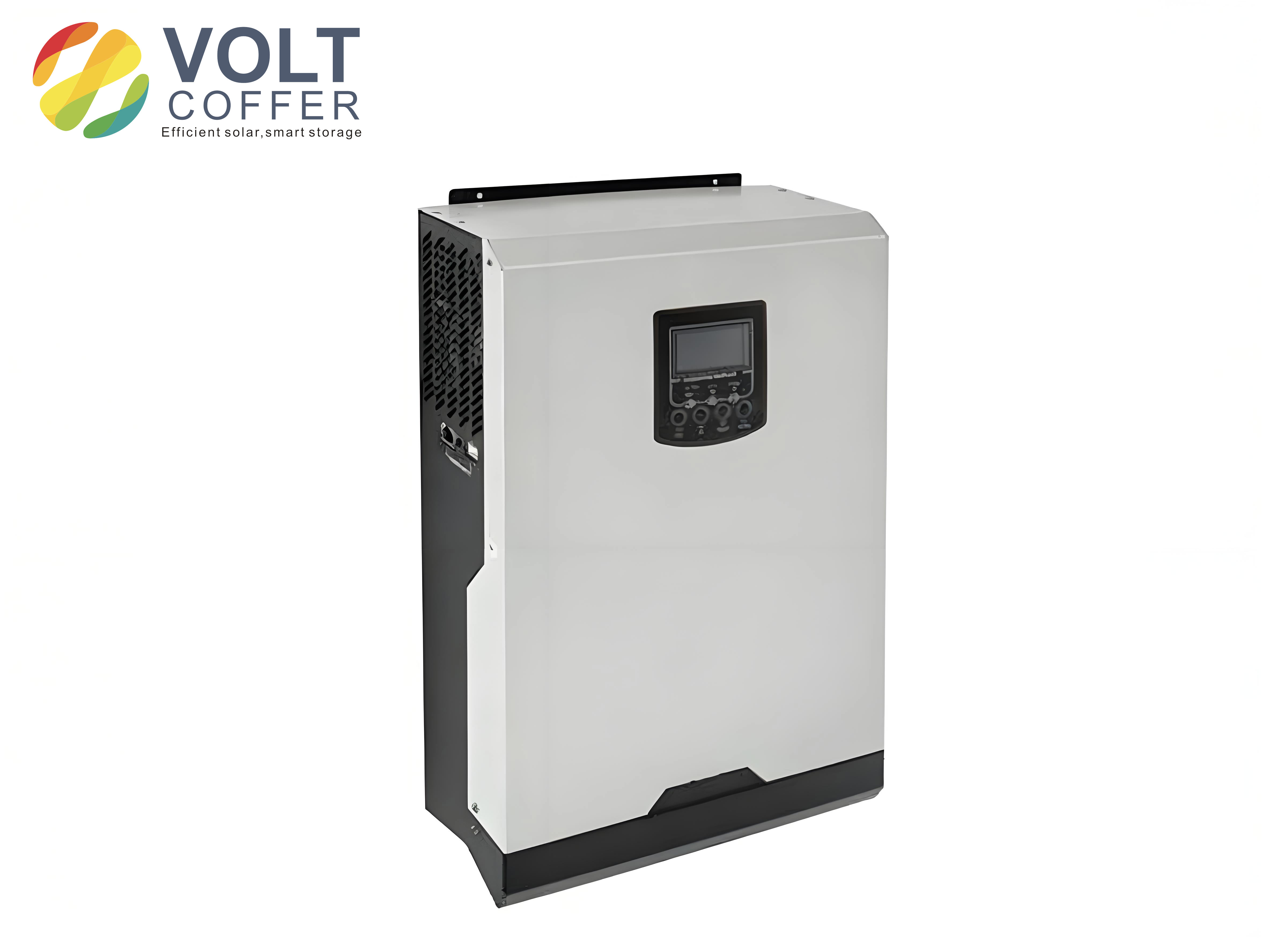
A representative example of the hardware class considered in this work is shown below.
During the experimental test, the inverter was connected to the grid through an isolation transformer and a variable grid impedance. The steady-state grid current waveform was clean, and the measured total harmonic distortion was below 3% at full load. The low-order harmonics measured in the experiment are summarized below. The table compares the state-feedback-only case with the full composite control strategy.
| Harmonic order | State feedback only | State feedback + feed-forward + repetitive |
| 3rd | 3.4% | 0.7% |
| 5th | 2.1% | 0.5% |
| 7th | 1.6% | 0.4% |
| 9th | 1.1% | 0.3% |
| THD | 5.1% | 2.2% |
I also studied the transient response of the composite controller. The current command was stepped from full load to half load. In a series repetitive controller, the reference signal itself passes through the \(z^{-N}\) delay, so the grid current begins to change only after one fundamental period. The error may remain visible for two or three additional periods because the periodic error accumulator needs time to converge. In the proposed embedded repetitive controller, the reference path is separated from the repetitive correction path. The grid current trackes the new command within about three fundamental cycles, and the transient overshoot is small because the state-feedback loop is well damped.
The following table gives a comparison among three strategies that are often used in grid-connected solar inverters.
| Criterion | Conventional PI | PI plus repetitive | Proposed composite control |
| Resonance damping | Poor without passive damping | Moderate | Good |
| Low-order harmonic rejection | Poor | Good | Excellent |
| Steady-state fundamental error | Finite | Nearly zero | Nearly zero |
| Transient response | Fast but oscillatory | One-cycle delay | Fast and well damped |
| DC-link ripple rejection | Poor | Moderate | Excellent |
| Grid voltage disturbance rejection | Poor | Moderate | Excellent |
| Implementation complexity | Low | Medium | Medium-high but manageable |
I define the total harmonic distortion of the grid current as
$$
\mathrm{THD} =
\frac{
\sqrt{\sum_{h=2}^{\infty} I_h^2}
}{
I_1
}
\times 100\%
$$
where \(I_1\) is the RMS value of the fundamental current and \(I_h\) is the RMS value of the \(h\)-th harmonic. In the final experiment the measured THD remained below 3% from 30% load to full load. The proposed feed-forward paths were especially useful when I intentionally increased the DC-link ripple by reducing the DC-link capacitance. Without DC-voltage feed-forward, the low-order harmonics increased sharply; with the feed-forward, the current spectrum remained almost unchanged.
Discussion of the Results
The results confirm that the resonant peak of the LCL filter is not the only obstacle to high-quality current injection in solar inverters. Even if the resonance is damped by state feedback, the low-order harmonics caused by dead-time, grid distortion, and DC-link ripple remain. The repetitive controller directly addresses these periodic disturbances. However, a repetitive controller alone is not sufficient because its inherent delay degrades the dynamic response. The embedded arrangement solves this problem.
One important practical aspect is the design of the phase compensator \(C(z)\). The LCL filter and the state-feedback loop introduce a frequency-dependent phase lag. If the compensator does not provide enough phase lead, the repetitive control loop can become unstable at certain frequencies. I tuned the phase lead \(m\) by inspecting the frequency response of \(C(z)P_{sc}(z)\). With \(m=2\), the product was close to unity in the frequency range from 50 Hz to about 1 kHz, which contains the most important harmonic orders. Higher harmonic orders have smaller amplitudes and are further attenuated by \(S(z)\).
The choice of the repetitive gain \(k_{rp}\) also involves a trade-off. A larger gain gives faster convergence of harmonic errors but reduces the stability margin. The value \(k_{rp}=0.85\) was found to provide a good compromise in the experimental prototype. It allowed the harmonic error to converge in about two or three fundamental cycles while maintaining a sufficient stability margin against grid impedance variation.
The state-feedback loop also improves robustness. The original LCL plant has a very high peak at the resonance frequency. This peak is undesirable because it can amplify switching noise and grid background harmonics. After pole placement, the closed-loop transfer function is smooth and has a nearly flat gain in the low-frequency range. This means that the repetitive controller sees a much easier plant to compensate. Furthermore, the state-feedback loop gives the system a predictable phase response, which simplifies the design of the repetitive compensator.
I also verified the behavior under a distorted grid voltage. When the grid voltage contained 3% of fifth harmonic and 2% of seventh harmonic, the proposed grid-voltage feed-forward path immediately reduced the corresponding current harmonics. The remaining harmonic error was then removed by the repetitive controller. The experimental results showed that the combined action was superior to either feed-forward or repetitive control used alone.
Design Procedure Summary
For engineers who want to implement the proposed strategy in other solar inverters, I suggest the following design procedure.
First, choose the LCL filter parameters so that the resonance frequency satisfies the usual constraint
$$
10f_0 < f_{\mathrm{res}} < 0.5 f_s
$$
Second, obtain the discrete-time model of the LCL plant at the sampling frequency. Third, select the desired closed-loop poles of the state-feedback system. The dominant poles should give a damping ratio between 0.7 and 0.9 and a natural frequency sufficiently lower than the LCL resonance frequency. The third pole is placed several times farther from the imaginary axis. Fourth, compute the state-feedback gain \(\boldsymbol{K}\) and the reference gain \(k_r\). Fifth, add the DC-voltage normalization and the partial grid-voltage feed-forward. Sixth, design the repetitive controller. Select \(N=f_s/f_0\), select \(Q(z)\) close to unity, select \(k_{rp}\), and design \(C(z)\) so that the stability condition is satisfied. Seventh, perform a simulation with a distorted grid and a DC-link ripple to verify the harmonic compensation. Finally, implement the controller on a prototype and measure the current THD and the transient response.
The following table summarizes the complete design procedure.
| Step | Action | Target |
| 1 | Modelling of LCL filter | Accurate state-space and transfer function |
| 2 | Pole placement | Damped resonance, fast settling |
| 3 | Reference feed-forward | Unity DC gain for current command |
| 4 | DC-voltage feed-forward | Decouple DC-link ripple |
| 5 | Grid-voltage feed-forward | Reject grid background distortion |
| 6 | Repetitive controller design | Periodic low-order harmonic rejection |
| 7 | Stability check | Satisfy the H-infinity condition |
| 8 | Simulation | Verify transient and steady-state performance |
| 9 | Experimental validation | Measure THD and dynamic response |
One of the most important conclusions I draw from this work is that harmonic compensation in grid-connected solar inverters cannot be solved by a single controller. Voltage feed-forward, state feedback, and repetitive control have complementary strengths. Feed-forward acts almost instantly but cannot eliminate every harmonic because the full grid-voltage cancellation path requires an impracticable differentiator. State feedback gives well-behaved plant dynamics and fast response but has no internal model of periodic disturbances. The repetitive controller provides the high periodic gain required for low-order harmonic suppression but has a delay that harms transient performance if placed in series with the reference. The composite structure combines these three elements so that each one does what it does best.
Conclusion
I have presented a composite control strategy for single-phase grid-connected solar inverters based on LCL filters. The method uses state-feedback pole placement to damp the LCL resonance, DC-voltage feed-forward decoupling to remove the influence of DC-link ripple, grid-voltage feed-forward to reject grid disturbance, and an embedded repetitive controller to suppress periodic low-order harmonics.
The state-feedback loop gives the current control system good damping and fast dynamic response. The DC-voltage feed-forward makes the inverter bridge gain independent of the measured DC-link voltage. The grid-voltage feed-forward reduces current harmonics caused by a distorted grid. The embedded repetitive controller provides high gain at multiples of the fundamental frequency, which eliminates the low-order harmonic errors caused by dead-time effects and other periodic disturbances.
I verified the proposed strategy through both simulation and laboratory experiments on a 2 kW solar inverter. The measured grid current THD was below 3% at full load, the low-order harmonics were strongly suppressed, and the transient response to a step change in the current command was fast. The results show that the composite controller is a practical and effective solution for high-performance grid-connected solar inverters. It combines the advantages of state feedback, feed-forward compensation, and repetitive control while avoiding the delay disadvantage of a series repetitive controller.