
My research focuses on the design, modeling, and optimization of a photovoltaic energy storage system for mobile agricultural applications. I also developed a portable telescopic solar panel bracket to support rapid deployment in complex outdoor environments. The proposed photovoltaic energy storage system can operate in both islanded and grid-connected modes, and it combines maximum power point tracking, battery charge management, hybrid power balancing, structural design, and reliability monitoring. The core objective is to establish an efficient and robust energy storage system that can be used for small-scale microgrids, electric field robots, and portable renewable energy devices. Throughout this work, I repeatedly considered the coupling between solar generation, battery storage, load demand, and grid interaction. My proposed energy storage system uses a lead-acid battery pack, a bidirectional DC-DC converter, a grid interface converter, and a load-side inverter. The energy management strategy maintains power balance and voltage stability while ensuring safe charging and discharging of the battery.
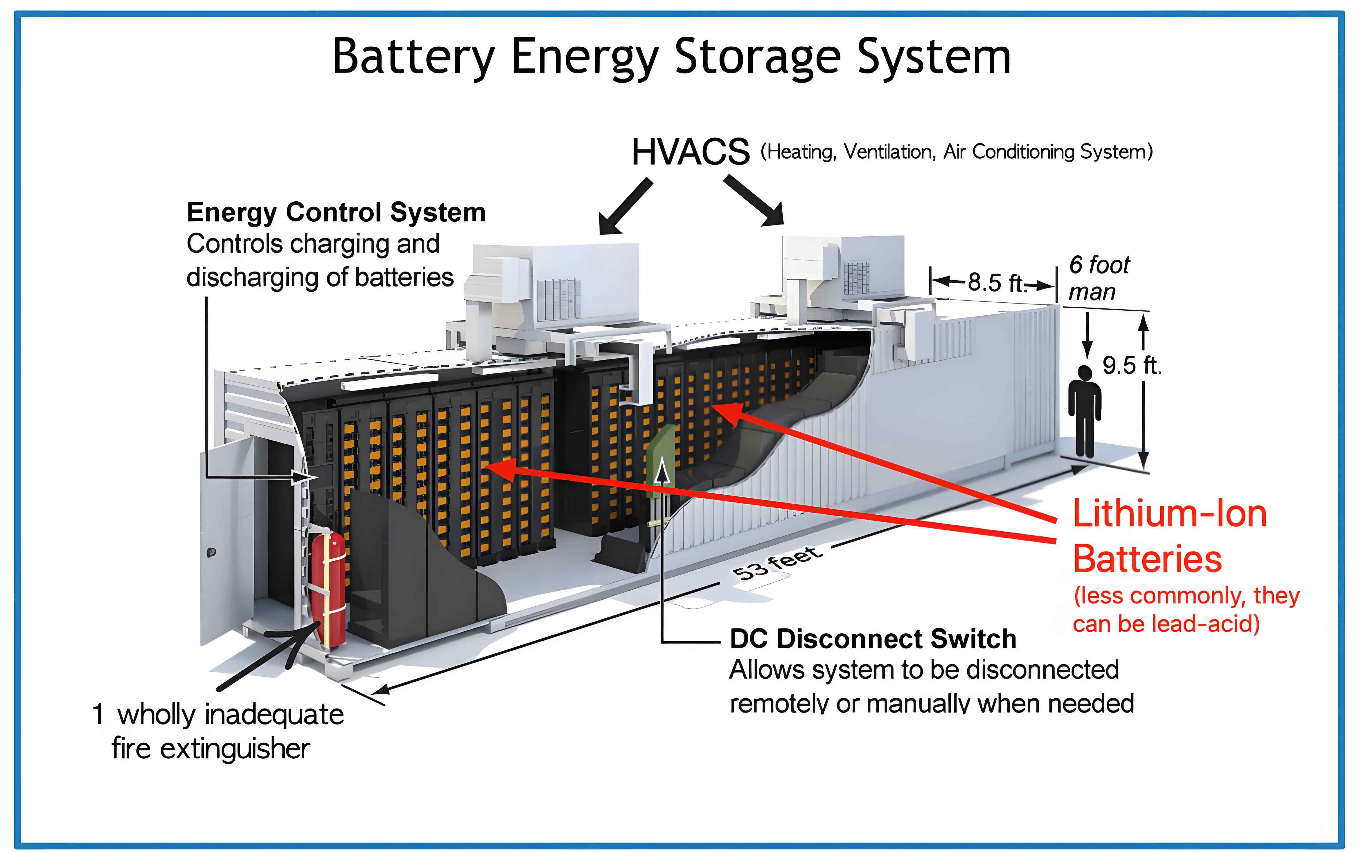
A representative layout of the proposed energy storage system is shown in the following illustration. The system links the photovoltaic array, the battery energy storage unit, the DC bus, the AC load, the DC load, and the external utility grid through controlled power converters.
1. Introduction and Application Background
The global energy landscape is shifting rapidly toward renewable sources, and solar energy has become one of the fastest growing technologies. In my work, I intend to support this transition by designing a photovoltaic energy storage system that can provide reliable power in rural, mobile, and grid-connected environments. The research originates from the need to power an intelligent daylily harvesting robot with solar electricity. That robot must operate in open fields, where grid access is not always available. I therefore designed a photovoltaic energy storage system with sufficient battery capacity and a solar array that can be quickly expanded through a portable support structure.
From the literature, I observed that many previous studies focus on either power electronics or structural supports, but few address the full system integration of photovoltaic energy storage, charging optimization, power sharing, structural adaptability, and condition monitoring. My work fills this gap by combining all of these elements. The energy storage system I designed is intended to handle both DC loads and AC loads, to smooth solar power fluctuations, and to maintain stable operation under changing irradiance and temperature. In addition, the portable bracket enables the deployment of twelve photovoltaic panels on top of a mobile robot, which significantly increases the available solar power without requiring a large permanent ground structure.
I reviewed energy storage technologies including pumped hydro, superconducting magnetic storage, supercapacitors, flywheels, vanadium redox flow batteries, lead-acid batteries, lithium batteries, and sodium-sulfur batteries. Table 1 summarizes typical parameters for several storage options. I observed that no single storage technology simultaneously provides high energy density, high power density, long cycle life, low cost, and low maintenance. For this reason, my proposed photovoltaic energy storage system is designed to be modular. It can be reconfigured with different battery chemistries, while the control strategies remain applicable.
| Storage technology | Power rating | Energy density (W·h/kg) | Power density (W/kg) | Cycle life | Efficiency (%) |
|---|---|---|---|---|---|
| Pumped hydro | 100 MW–200 MW | 0.5–1.5 | — | — | 70–85 |
| Superconducting magnetic | 10 kW–20 MW | 0.5–10 | 10⁷–10⁸ | >10⁵ | >96 |
| Supercapacitor | 10 kW–10 MW | 0.05–15 | 3000–4000 | >10⁵ | 90–95 |
| Flywheel | 5 kW–5 MW | 10–30 | >5000 | >10⁵ | 85–95 |
| Vanadium flow | kW–MW | 80–130 | 80–150 | >1200 | 75–80 |
| Lead-acid battery | 1 kW–50 MW | 30–50 | 75–300 | 500–1000 | 80–90 |
| Lithium battery | kW–MW | 75–200 | 200–315 | 500–10000 | 80–95 |
| Sodium-sulfur | kW–MW | 150–240 | 90–230 | 2500–6000 | 75–90 |
From this comparison, I concluded that lead-acid batteries remain a practical choice for small, low-cost photovoltaic energy storage systems. They are robust, widely available, and easy to recycle. Therefore, my main simulation uses a lead-acid battery model. The control algorithms, however, are not restricted to lead-acid chemistry; they can be adapted to lithium batteries as well. I also considered using supercapacitors to reduce battery stress, but for the intended agricultural robot, the additional complexity was not necessary. The energy storage system design therefore centers on a lead-acid battery pack with a bidirectional converter and a four-stage charging controller.
2. Photovoltaic Cell Modeling and Output Characteristics
I first developed an equivalent circuit model for the photovoltaic cell. The single-diode model contains a photocurrent source \(I_L\), a diode, a shunt resistance \(R_{sh}\), a series resistance \(R_s\), and a load resistance \(R\). The current-voltage relationship is written as
$$
I = I_L – I_0 \left[\exp\left(\frac{q(U + I R_s)}{A K T}\right)-1\right] – \frac{U + I R_s}{R_{sh}},
$$
where \(I_0\) is the diode reverse saturation current, \(q\) is the electron charge, \(A\) is the diode ideality factor, \(K\) is the Boltzmann constant, and \(T\) is the absolute temperature. To make the model useful for engineering simulation, I simplified this into a four-parameter engineering model:
$$
I = I_{sc} \left[1 – C_1 \left(\exp\left(\frac{U}{C_2 V_{oc}}\right)-1\right)\right],
$$
$$
C_1 = \left(1-\frac{I_m}{I_{sc}}\right)\exp\left(-\frac{V_m}{C_2 V_{oc}}\right),
$$
$$
C_2 = \frac{\left(\frac{V_m}{V_{oc}}-1\right)}{\ln\left(1-\frac{I_m}{I_{sc}}\right)}.
$$
Here \(I_{sc}\) is the short-circuit current, \(V_{oc}\) is the open-circuit voltage, \(I_m\) is the current at the maximum power point, and \(V_m\) is the voltage at the maximum power point. By introducing empirical compensation coefficients, I can calculate these four parameters for any irradiance \(S\) and temperature \(T\):
$$
I_{sc} = I_{sc,ref}\frac{S}{S_{ref}}\left(1+a\Delta T\right),
$$
$$
V_{oc} = V_{oc,ref}\left(1-b\Delta S+c\Delta T\right),
$$
$$
I_m = I_{m,ref}\frac{S}{S_{ref}}\left(1+a\Delta T\right),
$$
$$
V_m = V_{m,ref}\left(1-b\Delta S+c\Delta T\right).
$$
In these expressions, \(S_{ref}\) is the reference irradiance of 1000 W/m², \(\Delta T = T – T_{ref}\) is the temperature difference from the reference temperature, and \(a\), \(b\), \(c\) are empirical coefficients. I implemented this model in MATLAB/Simulink using a controlled current source. The photovoltaic module used in my simulations has an open-circuit voltage of 22 V, a short-circuit current of 5.8 A, a maximum power of 100 W, and a conversion efficiency of 17.8%.
| Parameter | Value |
|---|---|
| Maximum power | 100 W |
| Open-circuit voltage | 22 V |
| Short-circuit current | 5.8 A |
| Conversion efficiency | 17.8% |
The output characteristics show that irradiance strongly affects the short-circuit current, while temperature strongly affects the open-circuit voltage. I derived the conversion efficiency of the photovoltaic array as
$$
\eta = \frac{P_m}{P_{all}} = \frac{U_m I_m}{S K_{all}} \times 100\%,
$$
where \(K_{all}\) is the total area illuminated by sunlight. I found that the efficiency increases with the natural logarithm of irradiance, which explains why the energy storage system must include a tracking algorithm to keep the photovoltaic array at its maximum power point. I also modeled the temperature dependence of efficiency as
$$
\eta = \eta_0 \left[1-\alpha\left(T-T_0\right)\right],
$$
where \(\eta_0\) is the reference efficiency at 0°C and \(\alpha\) is the temperature coefficient. This relationship indicates that an increase of 10°C can reduce output power by several percent. Therefore, the energy storage system must not only maximize power extraction but also manage thermal effects in the power electronic converters.
3. Improved Maximum Power Point Tracking and Charging Control
Maximum power point tracking is essential for any photovoltaic energy storage system. I compared the incremental conductance method, the perturbation and observation method, and the constant voltage method. The conventional perturbation and observation method is simple but suffers from a trade-off between tracking speed and steady-state oscillation. If the step size is large, the tracking speed is high but the oscillation around the maximum power point is severe. If the step size is small, the oscillation is reduced but the tracking time becomes longer. To overcome this limitation, I proposed a variable-step-size perturbation and observation method, abbreviated as VSS-POM-MPPT. The reference voltage is updated as
$$
U_{ref}(k+1) = U_{ref}(k) + \alpha \frac{P(k)-P(k-1)}{U(k)-U(k-1)},
$$
where \(\alpha\) is an adjustable speed factor and \(k\) is the sampling index. When the working point is far from the maximum power point, the power difference is large, so the step becomes large and tracking is fast. When the working point approaches the maximum power point, the power difference becomes small, so the step becomes small and steady-state oscillation is reduced. I also introduced a small threshold \(\varepsilon\) to determine whether the voltage change is close to zero. If the voltage difference is below this threshold, the algorithm considers that the maximum power point has been reached and stops perturbing.
I implemented both the conventional perturbation and observation method and the proposed VSS-POM method in Simulink. Under constant irradiance of 1000 W/m² and a temperature of 25°C, my improved algorithm reached the maximum power point 0.008 seconds faster than the conventional algorithm. This corresponds to a speed improvement of 24.3%. I then tested the dynamic response under sudden irradiance changes and sudden temperature changes. When irradiance dropped from 1000 W/m² to 800 W/m², the improved algorithm tracked the new maximum power point in 0.021 seconds. When temperature rose from 25°C to 35°C, it tracked the new maximum power point in 0.025 seconds. These results confirm that the improved algorithm is fast and stable.
| MPPT Algorithm | Tracking time (s) | Steady-state oscillation | Speed improvement |
|---|---|---|---|
| Conventional P&O | 0.033 | Moderate | Baseline |
| VSS-POM | 0.025 | Small | 24.3% |
The energy storage system also needs a charging strategy that accounts for the random and intermittent nature of photovoltaic power. Traditional three-stage charging uses constant current, constant voltage, and floating charge. However, this approach does not fully consider the situation when the photovoltaic array is unable to supply enough current, or when the battery is deeply discharged. I therefore proposed a four-stage charging strategy based on the improved MPPT algorithm. The four stages are trickle pre-charge, constant current charge, constant voltage charge, and floating charge.
In the first stage, if the battery is deeply discharged, a small current of 0.05C is applied to slowly rebuild the electrochemical balance inside the battery. In the second stage, the battery is charged with a constant current. If the photovoltaic power is greater than the maximum acceptable battery power, the controller limits the charging current to the maximum allowed value and the photovoltaic array temporarily leaves the MPPT mode. If the photovoltaic power is lower than the battery limit, the system remains in MPPT mode and charges the battery at a safe current. In the third stage, the battery voltage reaches the preset maximum value. The controller then switches to constant voltage charging, and the charging current decays exponentially. In the fourth stage, when the charging current drops below a cutoff threshold, the system switches to floating charge. The floating voltage is lower than the constant voltage, so a small compensation current is maintained to offset self-discharge.
I experimentally validated the charging strategy by measuring voltage stabilization accuracy and current stabilization accuracy. The results show that the voltage stabilization accuracy is within ±0.4%, and the current stabilization accuracy is within ±0.8%. These values satisfy the national industry standards, which require voltage accuracy in the range ±0.5% to ±1% and current accuracy in the range ±1% to ±2%.
| Quantity | Measured accuracy | National standard | Result |
|---|---|---|---|
| Voltage stabilization | ±0.4% | ±(0.5%–1%) | Pass |
| Current stabilization | ±0.8% | ±(1%–2%) | Pass |
I also performed an outdoor charging experiment with a 12 V, 65 Ah lead-acid battery. The battery was charged from 11:00 to 15:00 under clear sky conditions. I recorded the charging voltage and current every 15 minutes. The measured curves clearly show the four operating regions: a gradual voltage rise during constant current charging, a plateau during constant voltage charging, an exponential current decay, and a final low-power floating stage. This agreement between the measured data and the proposed four-stage charging algorithm verifies that my energy storage system can safely and efficiently charge the battery using solar power.
4. Hybrid Energy Management and Optimal Load Balancing
I constructed a hybrid energy management system that integrates photovoltaic generation, battery energy storage, the AC utility grid, and DC/AC loads. The complete photovoltaic energy storage system includes a photovoltaic array with a boost converter, a bidirectional DC-DC converter connected to the battery, a bidirectional AC/DC converter connected to the grid, and a load-side three-phase inverter. The power balance equation for the system is
$$
P_{PV}(t) + P_{BESS}(t) = P_{DC\_load}(t) + P_{AC\_load}(t) + P_{grid}(t),
$$
where \(P_{PV}\) is the photovoltaic power, \(P_{BESS}\) is the battery power, and \(P_{grid}\) is positive when power is delivered to the grid and negative when power is absorbed from the grid. The battery energy storage system can operate in both charge and discharge modes. In my control architecture, the bidirectional DC-DC converter maintains the DC bus voltage at a reference value \(V_{dc}^*\). The battery reference current is calculated from the reference power divided by the battery voltage:
$$
I_{Bref} = \frac{P_{BDC,ref}}{V_B}.
$$
For the boost converter, I used a direct duty-cycle control law derived from the MPPT algorithm. The reference duty cycle is
$$
D_{ref}(k) = 1 – \frac{V_{PV,ref}(k)}{V_{dc,ref}(k)}.
$$
I also modeled the inductor and capacitor dynamics of the bidirectional converter:
$$
L\frac{di_L}{dt} = V_{batt} – (1-d)V_{dc\_link},
$$
$$
C\frac{dV_{dc\_link}}{dt} = (1-d)i_L – i_o,
$$
where \(d\) is the duty cycle, \(i_L\) is the inductor current, \(i_o\) is the output current, \(V_{batt}\) is the battery voltage, and \(V_{dc\_link}\) is the DC bus voltage. The battery state of charge is estimated using the generic battery model in MATLAB/Simulink. The model distinguishes between charging and discharging by using a control signal \(Sel(s)\), which is zero during discharge and one during charge.
I defined six operating modes for the AC/DC microgrid. These modes cover both grid-connected and islanded operation. Table 5 shows the mode definitions.
| Mode | Microgrid state | PV operation | Battery | Grid | AC/DC converter | Load |
|---|---|---|---|---|---|---|
| 1 | Grid-connected | MPPT | Charging | Inverter | Normal | Normal |
| 2 | Grid-connected | MPPT | Discharging | Rectifier | Normal | Normal |
| 3 | Islanded | Constant voltage | Off | Off | Off | Normal |
| 4 | Islanded | MPPT | Discharging | Off | Off | Normal |
| 5 | Islanded | MPPT | Charging | Off | Off | Normal |
| 6 | Islanded | MPPT | Discharging | Off | Off | Shedding |
In my energy management strategy, the battery state of charge is limited between 20% and 80%. When the battery state of charge reaches 80%, charging is stopped. When it drops below 20%, the battery is protected from further discharge. In grid-connected mode, if the photovoltaic power exceeds the load demand, the excess power first charges the battery. When the battery is full, the remaining power is delivered to the grid. In islanded mode, the battery is used to compensate for power shortages. If the photovoltaic power is insufficient and the battery cannot supply the demand, the system sheds low-priority loads to maintain the DC bus voltage.
I performed simulations in MATLAB/Simulink to verify the proposed energy management system. The irradiance profile varied over time between 600 W/m² and 1000 W/m². The simulation results show that the boost converter increases the photovoltaic voltage to the required DC bus level. The maximum power point efficiency reaches 98.3% at an irradiance of 1000 W/m². When irradiance increases, the photovoltaic current increases proportionally while the voltage remains almost constant. The battery current is negative during charging and positive during discharging. The state of charge increases from 70% to 70.2% when excess solar power is available, and decreases to 59.5% when the battery supplies the load. The DC bus voltage remains stable, with a fluctuation rate below 2%. The overall system efficiency is 95.7%, with most losses occurring in the switching devices.
I also simulated the load-side inverter. The three-phase voltage source inverter using sinusoidal pulse width modulation produces balanced AC voltages and currents. The current waveform is smooth when connected to the AC load. In islanded mode, the grid is disconnected, and the DC bus is maintained by the photovoltaic array and the battery. The simulation shows that the AC load remains powered during islanding because the battery supplies the missing power. The state of charge of the battery decreases gradually during islanded operation. This confirms that my energy storage system can provide uninterrupted power to critical loads even when the utility grid is unavailable.
5. Portable Telescopic Solar Panel Bracket Design
One of the main practical challenges for the mobile photovoltaic energy storage system is the limited installation area on top of the agricultural robot. I therefore designed a portable telescopic solar panel bracket. The bracket is a hidden, extendable structure that can store all photovoltaic panels within a compact housing when retracted, and then expand to expose twelve panels when needed. This design solves the problems of poor mobility, large occupied space, and difficult relocation encountered with conventional fixed solar brackets.
The bracket consists of a hollow housing, a lower movable frame, an upper movable frame, an electric push-rod mechanism, pulley systems, slide rails, gear-rack transmission, and a set of linkage rods. The electric push rod is installed in the middle of the housing. When the push rod extends, it drives a scissor-like linkage mechanism. The linkage rods push the lower movable frame outward along T-shaped guide slots. When the lower frame reaches its end position, the gear-rack mechanism drives the upper frame to slide further outward. The deployment sequence is therefore divided into two stages. In the first stage, the electric push rod expands the lower frame. In the second stage, a travel switch triggers the gear-rack mechanism and expands the upper frame. The total deployment time is less than 30 seconds. The total length after complete extension is 4.464 m, the width is 1.964 m, and the height is 0.195 m. The wall thickness is 3 mm.
I selected 6061 aluminum alloy as the main material for the bracket because it offers a good balance between strength, weight, and corrosion resistance. The finite element model uses the following material properties: Young’s modulus \(E = 68.9\) GPa, Poisson’s ratio \(\nu = 0.33\), density \(\rho = 2700\) kg/m³, and yield strength around 240 MPa after T6 treatment.
| Material property | Value |
|---|---|
| Material | 6061 aluminum alloy |
| Young’s modulus | 68.9 GPa |
| Poisson’s ratio | 0.33 |
| Density | 2700 kg/m³ |
| Yield strength | 240 MPa |
I imported the three-dimensional model into the simulation platform and applied the self-weight of 12 photovoltaic panels. Each panel has a mass of 10 kg, so the total applied load is 1200 N. I also considered the horizontal thrust and tension transmitted through the electric telescopic structure during the expansion and retraction processes. The finite element equilibrium equation for each element can be written as
$$
K^e u^e = P^e,
$$
where \(K^e\) is the element stiffness matrix, \(u^e\) is the element displacement vector, and \(P^e\) is the element force vector. After solving the global displacement field, the stress and strain are calculated using
$$
\sigma = D B u^e,
$$
where \(D\) is the elasticity matrix and \(B\) is the strain-displacement matrix. The safety factor at any point is defined as
$$
n = \frac{\sigma_y}{\sigma_{vonMises}},
$$
where \(\sigma_y\) is the yield strength and \(\sigma_{vonMises}\) is the equivalent von Mises stress.
The finite element results show that the maximum deformation of the upper bracket is 1.208 mm. This displacement is small enough to avoid affecting the normal operation of the photovoltaic panels. The minimum safety factor is 4.2 for the upper bracket, which is much larger than the required minimum safety factor of 1.5. I also analyzed the electric telescopic linkage structure, especially the outer strut, which carries the highest load during deployment. The von Mises stress remains below the yield strength, and the safety factor is sufficient. The simulation thus verifies that the structural design is reliable.
| Component | Maximum displacement | Minimum safety factor | Requirement |
|---|---|---|---|
| Upper support frame | 1.208 mm | 4.2 | <2 mm, >1.5 |
| Electric telescopic linkage | Within elastic range | Sufficient | >1.5 |
In addition to static loading, I considered the practical constraints of repeated deployment and folding in the field. The electric push rod and the gear-rack mechanism are designed to operate within their stroke limits, and the T-shaped guide slots ensure smooth movement. The bracket can be fully retracted into the housing, protecting the photovoltaic panels from wind, dust, and mechanical damage during transport. When the robot moves to a new field, the operator can deploy the photovoltaic energy storage system again in less than 30 seconds. This structural innovation significantly improves the space utilization and mobility of the solar power generation system.
6. Intelligent Operation and Reliability Assessment for the Energy Storage System
The outdoor operation of a photovoltaic energy storage system exposes the solar panels to various risks, including short-circuit faults, open-circuit faults, partial shading, dust accumulation, and aging. These conditions can reduce the output power and damage the battery charging process. I therefore developed a condition assessment method based on combined weighting and Markov chain Monte Carlo simulation. The proposed method continuously monitors key electrical indicators and predicts the probability of failure for each photovoltaic string. This allows the energy storage system to receive early warnings before a complete failure occurs.
I selected four assessment indicators: current ratio \(X_1\), voltage ratio \(X_2\), fill factor \(X_3\), and power ratio \(X_4\). They are defined as
$$
X_1 = \frac{I_m}{I_{mp}},
$$
$$
X_2 = \frac{U_m}{U_{mp}},
$$
$$
X_3 = FF = \frac{U_m I_m}{U_{oc} I_{sc}},
$$
$$
X_4 = \frac{P_m}{P_{mp}},
$$
where \(I_m\) and \(U_m\) are the measured current and voltage at the maximum power point, \(I_{mp}\) and \(U_{mp}\) are the expected values under normal conditions, and \(P_m\) and \(P_{mp}\) are the measured and expected maximum powers. These indicators can distinguish between normal operation, shading, aging, dust, and circuit faults. For example, a short-circuit fault changes the open-circuit voltage, while an open-circuit fault significantly reduces the short-circuit current. Aging and shading both reduce the maximum power, but their effects on the fill factor are different.
I normalized the raw data using the range method:
$$
x_{ij}^* = \frac{x_{ij} – m_j}{M_j – m_j},
$$
where \(m_j = \min_i x_{ij}\) and \(M_j = \max_i x_{ij}\). After normalization, I combined a subjective weighting method with an objective weighting method. The subjective weights are obtained using the G1 method. In the G1 method, the decision-maker first ranks the indicators according to importance, then gives the ratio \(r_k\) between adjacent indicators:
$$
r_k = \frac{w_{k-1}}{w_k}.
$$
Using the ratios, the final subjective weight is calculated as
$$
w_m = \left(1+\sum_{k=2}^{m}\prod_{i=k}^{m} r_i\right)^{-1},
$$
$$
w_{k-1} = r_k w_k.
$$
The objective weights are computed using the entropy weight method. The entropy \(E_j\) of the \(j\)-th indicator is
$$
E_j = -\frac{1}{\ln n}\sum_{i=1}^{n} p_{ij}\ln p_{ij},
$$
$$
p_{ij} = \frac{x_{ij}}{\sum_{i=1}^{n} x_{ij}},
$$
$$
w_j = \frac{1-E_j}{\sum_{j=1}^{m}(1-E_j)}.
$$
I then multiplied the subjective weight \(w_{1j}\) and the objective weight \(w_{2j}\), and normalized the result to obtain the combined weight:
$$
w_j = \frac{w_{1j} w_{2j}}{\sum_{k=1}^{m} w_{1k} w_{2k}}.
$$
Using the combined weights, I calculated the score \(p_i\) for each photovoltaic string:
$$
p_i = \sum_{j=1}^{m} w_j x_{ij}^*.
$$
After normalizing these scores, the failure probability of each string is estimated as
$$
p_{ai} = \frac{p_i}{\sum_{i=1}^{n} p_i}.
$$
To simulate the dynamic and uncertain behavior of photovoltaic faults, I used the Markov chain Monte Carlo method with Gibbs sampling. I defined three random variables to represent the fault type, the faulty string location, and the number of faulty strings. The fault type \(S_1\) is generated from a discrete distribution:
$$
S_1 =
\begin{cases}
1, & x_1 < p_1,\\
2, & p_1 \le x_1 < p_1+p_2,\\
3, & p_1+p_2 \le x_1 < 1,
\end{cases}
$$
where \(p_1\), \(p_2\), and \(p_3\) are the probabilities of shading, aging, and dust, respectively. In my analysis, the probabilities are set as 42%, 21%, and 42% for shading, aging, and dust. The faulty string location is updated using a Markov chain. At each iteration, I update one string’s failure state while keeping all other string states fixed. This Gibbs sampling procedure produces a sequence of binary state vectors that converges to the target posterior distribution. After many iterations, the failure probability of a string is estimated by counting the number of times it appears in a failed state:
$$
\hat{p}_{ai} = \frac{FT_i}{N},
$$
where \(FT_i\) is the number of Monte Carlo trials in which string \(i\) fails, and \(N\) is the total number of trials. In my simulation, I used 2000 Monte Carlo trials. The convergence of the failure probability is good. The estimated failure probability intervals are consistent with the measured data, and the accuracy is above 90%.
I also defined four efficiency status intervals for the photovoltaic array. If the relative efficiency \(\eta’\) is between 0.8 and 1.0, the array is classified as excellent. If it is between 0.6 and 0.8, the array is classified as acceptable. If it is between 0.5 and 0.6, the array is considered degraded, and if it is below 0.5, maintenance is required. Table 7 summarizes the fault probabilities and relative efficiencies used in the Monte Carlo simulation.
| Fault type | Probability (%) | Relative efficiency (%) |
|---|---|---|
| Normal | — | 87.9 |
| Shading | 42 | 67.1 |
| Aging | 21 | 68.9 |
| Dust | 42 | 67.9 |
I applied the proposed assessment method to a photovoltaic array divided into five sub-arrays, labeled PV1 to PV5. Each sub-array has twelve strings. The evaluation results are shown in Table 8. PV1, PV3, PV4, and PV5 are classified as excellent because their most frequent relative efficiency intervals are all above 0.8. PV2 is classified as acceptable because its efficiency interval is around 0.78 to 0.80. This indicates that PV2 may have dust accumulation, slight shading, or early aging. The method successfully identifies this condition and suggests that preventive maintenance is needed.
| Array | Most frequent efficiency interval | Assessment result |
|---|---|---|
| PV1 | (0.819–0.841) | Excellent |
| PV2 | (0.779–0.801) | Acceptable |
| PV3 | (0.809–0.828) | Excellent |
| PV4 | (0.801–0.839) | Excellent |
| PV5 | (0.801–0.839) | Excellent |
The combination of G1 weighting and entropy weighting makes the assessment robust. The subjective weights capture expert knowledge, while the objective weights reflect the information contained in the data. The Markov chain Monte Carlo approach provides a probabilistic rather than deterministic evaluation. This is particularly useful for an energy storage system that operates in changing weather conditions. By using Gibbs sampling, I can update the failure probability as new measurement data become available. This creates a dynamic condition monitoring framework for the photovoltaic energy storage system.
7. Conclusions and Outlook
In this research, I designed and optimized a photovoltaic energy storage system and developed a portable telescopic solar panel bracket. The main conclusions are summarized as follows.
First, I established an accurate photovoltaic cell model and analyzed the output characteristics under different irradiance and temperature conditions. I then proposed a variable-step perturbation and observation MPPT algorithm. Compared with the conventional method, my improved algorithm reduces the tracking time by 0.008 seconds and improves the tracking speed by 24.3%. The algorithm also reduces the oscillation around the maximum power point. This improvement is important for the dynamic performance of the energy storage system under rapidly changing environmental conditions.
Second, I proposed a four-stage battery charging strategy based on the improved MPPT algorithm. The strategy includes trickle pre-charge, constant current charge, constant voltage charge, and floating charge. Experimental results show that the voltage stabilization accuracy is ±0.4% and the current stabilization accuracy is ±0.8%, both of which meet the national standards. The outdoor charging test verified that the actual charging process closely matches the designed four-stage algorithm.
Third, I designed a hybrid energy management system for both islanded and grid-connected operation. The system coordinates the photovoltaic array, battery energy storage, AC utility grid, and DC/AC loads. The simulation results show that the DC bus voltage fluctuation is less than 2% and the overall system efficiency is 95.7%. The system can switch smoothly between charging and discharging modes, and the battery state of charge remains within the safe range from 20% to 80%.
Fourth, I designed a portable telescopic solar panel bracket that can hold twelve photovoltaic panels. The bracket uses an electric push rod, linkage mechanisms, slide rails, and a gear-rack transmission. The total deployment time is less than 30 seconds. Finite element analysis shows that the maximum displacement is less than 2 mm and the minimum safety factor is greater than 1.5, satisfying the structural requirements. This bracket is particularly suitable for mobile photovoltaic energy storage systems such as agricultural robots and portable microgrids.
Fifth, I developed a smart condition assessment method using combined weights and Markov chain Monte Carlo simulation. The method selects four key electrical indicators and calculates the failure probability of each photovoltaic string. The evaluation results are highly consistent with measured data, and the accuracy exceeds 90%. This monitoring framework can detect abnormal states such as shading, dust, aging, and circuit faults in real time, enabling predictive maintenance and improving the reliability of the photovoltaic energy storage system.
There are several directions for future work. I plan to integrate supercapacitors with lead-acid batteries or lithium batteries to form a hybrid energy storage system, which can improve the transient response and reduce battery stress. I also intend to apply the proposed control strategies to a physical prototype and test them under more extreme weather conditions. The portable bracket can be further optimized using topology optimization and lightweight design methods. Finally, the condition assessment framework can be extended with machine learning algorithms and internet-of-things sensors to create a fully autonomous monitoring platform. By continuously improving the design, control, and maintenance of photovoltaic energy storage systems, I hope to contribute to the widespread adoption of renewable energy in mobile and off-grid applications.