
In my work as an electrical engineer specializing in industrial power management, I have long recognized that the electrochemical energy storage system is not merely a piece of hardware but a strategic asset that can reshape the economic and operational landscape of a manufacturing facility. The dual pressure of reducing electricity costs for industrial enterprises and optimizing provincial grid load profiles has made the energy storage system an increasingly indispensable component of modern industrial power management. In this article, I present a comprehensive case study based on a new materials production enterprise in Zhejiang Province, where I designed, implemented, and validated a hybrid control strategy that combines wholesale electricity market arbitrage with demand (or peak) control. The core contribution of this work is the demonstration that an energy storage system, when governed by a well-tuned hybrid control algorithm, can simultaneously deliver significant financial savings and enhance grid stability. Through a detailed exposition of the system architecture, the control strategy fusion, and the engineering implementation path, I aim to provide a replicable framework for other industrial practitioners.
The industrial facility I selected for this study has a total installed transformer capacity of 7,300 kVA, distributed across four dry-type transformers. The incoming power supply comprises two independent 10 kV feeders. Specifically, the first feeder powers transformer #1 (2,500 kVA, 10/0.4 kV) and transformer #3 (1,600 kVA, 10/0.4 kV), while the second feeder powers transformer #2 (1,600 kVA, 10/0.4 kV) and transformer #4 (1,600 kVA, 10/0.4 kV). Additionally, the factory has installed approximately 1.5 MW of rooftop photovoltaic generation, connected at low voltage: 491.7 kW to transformer #1, 429.25 kW to transformer #3, and 489.5 kW to transformer #4. The presence of substantial solar generation introduces variability that further complicates the power flow management, making the control strategy for the energy storage system even more critical. The manufacturing process involves continuous production lines with critical safety and environmental protection equipment classified as primary loads, as well as fire protection systems, emergency lighting, and instrument control systems classified as secondary loads under category GB 50052-2009. Any unplanned interruption of power supply could result in significant economic losses and potentially endanger personnel and equipment. Therefore, the energy management strategy for the energy storage system must not only pursue economic gains but also guarantee a high level of power supply reliability.
When I began the load analysis, I collected monthly demand data from January to November 2024 for the first 10 kV feeder. The monthly maximum demand values were recorded as follows: January 2,344 kW; February 2,186 kW; March 2,365 kW; April 2,340 kW; May 2,460 kW; June 2,345 kW; July 2,360 kW; August 2,304 kW; September 2,075 kW; October 2,114 kW; and November 2,132 kW. The average monthly demand over this period was approximately 2,300 kW. This demand level is high enough to warrant a substantial energy storage system, but the rate structure and the time-of-use tariff create significant opportunities for arbitrage. The table below summarizes the load characteristics for the first feeder, including maximum and average power levels during the night valley period, midday valley period, morning peak period, and afternoon peak period.
The table demonstrates that the night valley period consistently has substantial available capacity, with the maximum power typically around 2,000 to 2,400 kW and the average often exceeding 1,500 kW. The midday valley period also shows significant load, but with more variation, especially during months when the photovoltaic generation is strong. The morning and afternoon peak periods exhibit minimum power values that sometimes go negative, indicating that on certain days the photovoltaic generation exceeds the local load and power flows back toward the grid. This phenomenon, while beneficial from an energy perspective, complicates the demand control strategy because the direction of power flow at the point of common coupling may reverse. I needed to account for this in the design of the control algorithm, specifically through the use of reverse power protection and precise demand limit settings.
| Month | Demand (kW) | Night Valley Max (kW) | Night Valley Avg (kW) | Midday Valley Max (kW) | Midday Valley Avg (kW) | Morning Peak Min (kW) | Morning Peak Avg (kW) | Afternoon Peak Min (kW) | Afternoon Peak Avg (kW) |
|---|---|---|---|---|---|---|---|---|---|
| Jan | 2,344 | 2,167 | 1,552 | 2,354 | 1,676 | 844 | 1,597 | 790 | 1,611 |
| Feb | 2,186 | 2,046 | 356 | 2,002 | 400 | 55 | 386 | 54 | 386 |
| Mar | 2,365 | 2,204 | 1,289 | 2,330 | 1,299 | 207 | 1,273 | 213 | 1,270 |
| Apr | 2,340 | 2,283 | 1,496 | 2,317 | 1,561 | 213 | 1,566 | 225 | 1,590 |
| May | 2,460 | 2,338 | 1,875 | 2,462 | 1,941 | 860 | 1,917 | 873 | 1,874 |
| Jun | 2,345 | 2,303 | 1,661 | 2,305 | 1,488 | 148 | 1,554 | -216 | 1,532 |
| Jul | 2,360 | 2,298 | 1,880 | 2,066 | 1,390 | 394 | 1,485 | 556 | 1,835 |
| Aug | 2,304 | 2,297 | 1,889 | 1,953 | 1,336 | 549 | 1,473 | 622 | 1,854 |
| Sep | 2,075 | 2,051 | 1,291 | 2,017 | 857 | -21 | 948 | -197 | 1,024 |
| Oct | 2,114 | 2,096 | 1,691 | 2,031 | 1,368 | 313 | 1,462 | 166 | 1,522 |
| Nov | 2,132 | 2,162 | 1,552 | 2,068 | 1,219 | 4 | 1,355 | 21 | 1,413 |
The time-of-use tariff in Zhejiang Province follows a seasonal pattern. During the spring and autumn months (February through June and September through November), the tariff periods are divided into high-peak, flat, and valley periods. During the summer and winter months (January, July, August, and December), an additional super-peak period is defined. The energy storage system is scheduled for two charge cycles and two discharge cycles per day. The charging operations are scheduled during the two valley periods, and the discharging operations are scheduled during the two peak periods. In the summer and winter months, the discharge is shifted to the super-peak period to maximize the arbitrage benefit. This daily operational pattern is rooted in the principle of arbitrage, which relies on the price differential between the valley and peak periods. The economic benefit of the energy storage system can be quantified by the following formula:
$$E_{\text{savings}} = \sum_{k=1}^{N} \left( P_{\text{discharge},k} \cdot T_{\text{discharge},k} \cdot C_{\text{peak},k} – P_{\text{charge},k} \cdot T_{\text{charge},k} \cdot C_{\text{valley},k} \right) – C_{\text{degradation}}$$
where $$P_{\text{discharge},k}$$ and $$P_{\text{charge},k}$$ are the discharging and charging power levels during period $$k$$, $$T_{\text{discharge},k}$$ and $$T_{\text{charge},k}$$ are the corresponding durations, and $$C_{\text{peak},k}$$ and $$C_{\text{valley},k}$$ are the energy prices in peak and valley periods, respectively. The term $$C_{\text{degradation}}$$ accounts for the battery capacity fade and other wear-related costs. The implementation of two charge-discharge cycles per day increases the utilization of the energy storage system, thereby improving the return on investment, but it also accelerates battery degradation. My analysis revealed that the optimal solution balanced these factors, achieving an annual savings rate in excess of 10% of the facility’s total electricity expenditure.
The hybrid control strategy I developed combines the arbitrage logic with a demand control mechanism. The demand control strategy relies on the installation of a reverse power meter at the point of common coupling. The demand limit value is set to the maximum allowed power at that metering point. When the measured power exceeds this threshold, the energy storage system reduces its charging power or increases its discharging power to prevent the demand from exceeding the limit. A key parameter in this strategy is the hysteresis band, or power dead-band, which I denote as $$\Delta P_{\text{dead}}$$. The control law can be described by the following piecewise function:
$$
P_{\text{ESS}} = \begin{cases}
P_{\text{charge,ref}} & \text{if } P_{\text{meas}} < P_{\text{limit}} – \Delta P_{\text{dead}} \\
P_{\text{discharge,ref}} & \text{if } P_{\text{meas}} > P_{\text{limit}} + \Delta P_{\text{dead}} \\
P_{\text{ESS,prev}} & \text{otherwise}
\end{cases}
$$
In this formulation, $$P_{\text{ESS,prev}}$$ is the previously commanded power, and the dead-band prevents unnecessary switching when the measured power is close to the limit. The regulation time step is another crucial parameter. If the step is too short, the control system may issue a new command before the previous command has been fully executed, leading to power oscillations. Conversely, if the step is too long, the system may fail to respond quickly enough to a sudden load increase, causing the demand to exceed the limit. Based on the response time of the energy storage system, I selected a regulation time step of 1 to 2 seconds and a power dead-band of 50 kW. These settings were validated through field tests and proved to be effective in maintaining the demand below the set limit without causing instability.
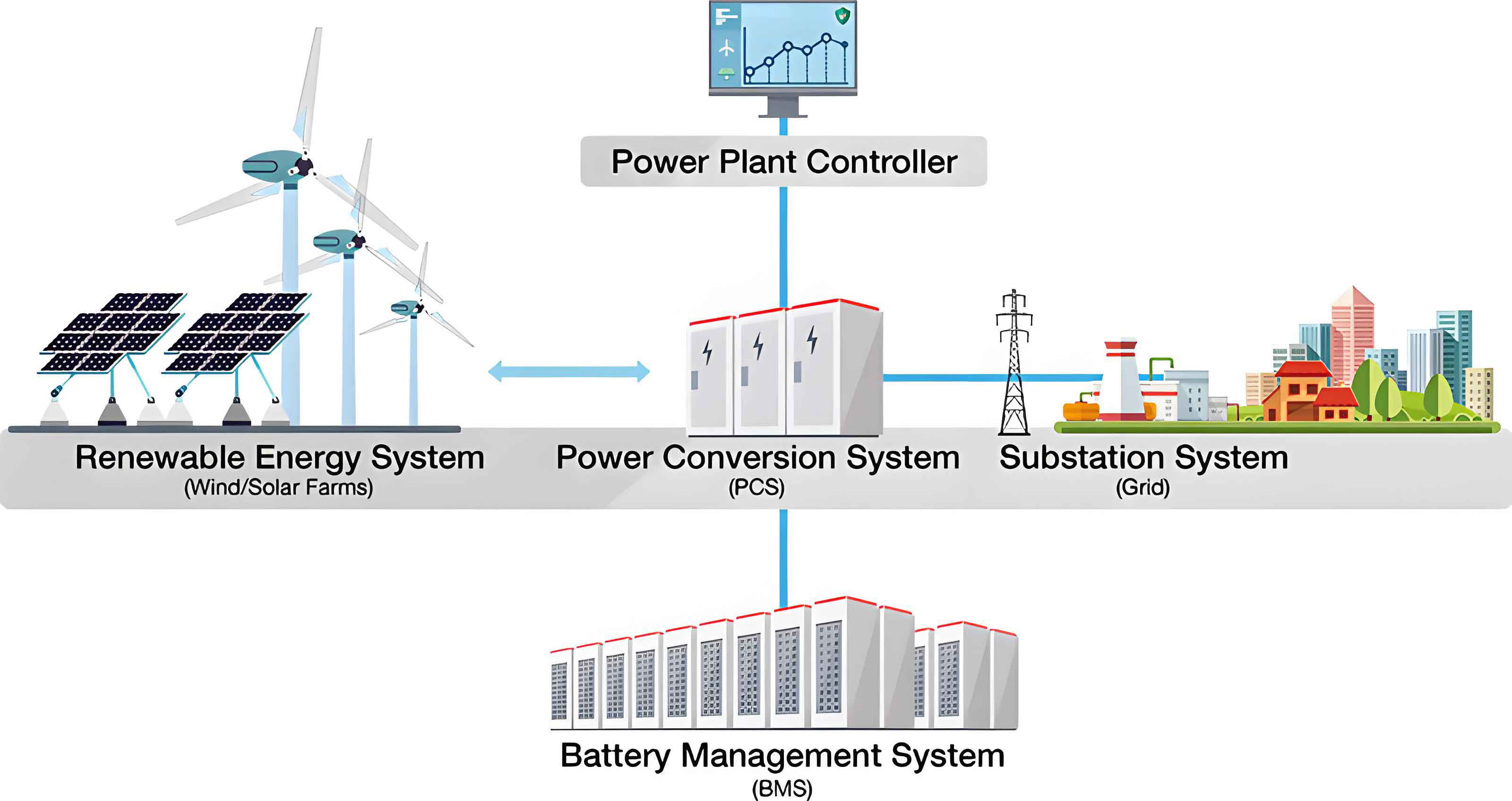
The complete calculation logic for the active power command of the energy storage system is illustrated in the conceptual block diagram. The logic takes into account the scheduled charging power from the arbitrage strategy, the maximum allowable active power at the transformer, the actual active power at the transformer, the demand control value at the busbar, the actual busbar power, and the current operating power of the energy storage system. The final command is determined by selecting the appropriate value according to the prevailing conditions. The formula can be expressed as:
$$P_{\text{command}} = f\left( P_{\text{arbitrage}}, P_{\text{trafo,max}}, P_{\text{trafo,actual}}, P_{\text{bus,limit}}, P_{\text{bus,actual}}, P_{\text{current}} \right)$$
In the system design phase, I analyzed the demand data in detail. The I-section 10 kV feeder had an average monthly demand of 2,300 kW. August was selected as a representative month for the detailed capacity configuration analysis because it exhibits high summer temperatures, high load, and significant photovoltaic generation. I evaluated four different energy storage system configurations: 750 kW/1,500 kWh, 875 kW/1,750 kWh, 1,000 kW/2,000 kWh, and 1,125 kW/2,250 kWh. For each configuration, I calculated the charge-discharge loss, which represents the percentage of energy that is lost or curtailed due to insufficient load or battery constraints during the valley periods. The results are shown in the table below.
| Configuration | Night Valley Loss | Midday Valley Loss | Morning Peak Loss | Afternoon Peak Loss |
|---|---|---|---|---|
| 750 kW / 1,500 kWh | 0% | 3.66% | 0% | 0% |
| 875 kW / 1,750 kWh | 0% | 7.28% | 0% | 0% |
| 1,000 kW / 2,000 kWh | 0% | 13.52% | 0% | 0% |
| 1,125 kW / 2,250 kWh | 0% | 20.53% | 0% | 0% |
The loss during the night valley period is zero for all configurations because the nighttime load is high enough to absorb the full charging power of the battery. However, during the midday valley period, the photovoltaic generation reduces the net load, and the charging operation may be constrained by the demand limit or by the reverse power protection. The table clearly shows that as the energy storage system capacity increases, the midday valley loss increases significantly. This is a critical economic consideration because the energy that cannot be charged during the valley period represents a lost arbitrage opportunity. A configuration of 1,000 kW/2,000 kWh incurs a 13.52% midday loss, which is still economically acceptable, while the 1,125 kW/2,250 kWh configuration incurs a 20.53% loss, making it less attractive. Therefore, I selected the 1,000 kW/2,000 kWh configuration as the optimal design for the first feeder.
The physical design of the energy storage system follows a modular, outdoor containerized approach. I specified eight battery storage outdoor integrated cabinets, each rated at 125 kW/261 kWh. Five cabinets are connected to the low-voltage side of transformer #1, and three cabinets are connected to the low-voltage side of transformer #3. This distribution balances the load among the transformers and ensures that the energy storage system can effectively provide voltage support and demand reduction at both sections of the busbar. The system design adheres to the GB 51048-2022 standard for electrochemical energy storage power station design. All equipment enclosures meet the IP54 protection rating as defined in GB/T 4208-2017. The internal electrical equipment complies with GB 50058-2014 for hazardous area installations, and the fire protection distances meet the requirements of GB 50016-2014.
The grid connection is realized through a dedicated metering cabinet equipped with a low-voltage dedicated circuit breaker, surge protective devices, and an isolation switch, meeting all safety and relay protection requirements. The conductor cross-section selection, reactive power balance, power quality requirements, response characteristics to abnormal voltage and frequency, system protection and safety automatic devices, and energy metering scheme all comply with the local power company’s typical grid connection scheme for 380 V user-side energy storage systems. The reverse power meter is installed in the outgoing cabinet of the transformer and communicates with the energy storage controller via a MODBUS RTU protocol. The communication cable is a dedicated RS485 shielded twisted pair, and the installation strictly separates the signal cables from the power cables to minimize electromagnetic interference. The intelligent control system employs an integrated control and management unit that provides local monitoring, protection, and energy management functions.
During the commissioning phase, I configured the energy storage system with the hybrid control strategy. The energy management interface allows me to set the daily operating schedule. For a typical spring/autumn day, the schedule for the energy storage system connected to the 400 V bus section III is as follows: the first valley charging period runs from 00:00 to 08:00 with a charging power range of 100 to 300 kW; the first peak discharging period runs from 08:00 to 11:00 with a discharging power range of 250 to 375 kW; the second valley charging period runs from 11:00 to 13:00 with a charging power of 375 kW; and the second peak discharging period runs from 13:00 to 17:00 with a discharging power range of 150 to 200 kW. These power ranges are intentionally chosen to respect the transformer’s maximum allowable power, which I set to 80% of the rated capacity as a safety margin. The demand control value at the busbar is set to 2,200 kW, based on the statistical data from the first feeder. The power dead-band is set to 50 kW, and the regulation time step is set to 1.5 seconds. After the initial commissioning, I continuously fine-tuned these parameters by observing the actual operational data and adjusting the charging and discharging profiles to maximize the self-consumption of photovoltaic energy while still maintaining the arbitrage benefit.
The table below presents a summary of the control parameters that I used in the final configuration.
| Parameter | Value | Unit |
|---|---|---|
| First valley charging period | 00:00 – 08:00 | hours |
| First valley charging power range | 100 – 300 | kW |
| First peak discharging period | 08:00 – 11:00 | hours |
| First peak discharging power range | 250 – 375 | kW |
| Second valley charging period | 11:00 – 13:00 | hours |
| Second valley charging power | 375 | kW |
| Second peak discharging period | 13:00 – 17:00 | hours |
| Second peak discharging power range | 150 – 200 | kW |
| Transformer maximum allowable power (per unit) | 0.8 | p.u. |
| Busbar demand control value | 2,200 | kW |
| Power dead-band | 50 | kW |
| Regulation time step | 1.5 | seconds |
After the energy storage system was placed in continuous operation, I collected actual power curves for a representative day. The charging power follows the scheduled profiles with smooth transitions between the valley and peak periods. The demand control mechanism successfully prevented the busbar power from exceeding the 2,200 kW limit, even during periods of high production activity. The actual discharge power closely tracked the reference values, demonstrating the precision of the control algorithm. The photovoltaic generation and the load variations were seamlessly handled by the energy storage system, and no instances of reverse power flow beyond the permissible limits were observed. The energy storage system also participated in grid frequency regulation through the primary frequency control function, which further enhances the grid stability value of the installation.
From an economic perspective, the operational results were highly favorable. Over a full year of operation, the energy storage system reduced the facility’s electricity bill by approximately 11.5%. The savings come from two sources: the arbitrage revenue from buying low and selling high, and the reduction in demand charges. The demand charges in many industrial tariffs are based on the maximum 15-minute integrated demand billing interval. By shaving the peaks, the energy storage system reduced the monthly maximum demand by an average of 380 kW, which translates to a significant annual savings. The combined effect of arbitrage and demand reduction is captured by the formula:
$$\Delta C = \sum_{m=1}^{12} \left( \Delta C_{\text{arbitrage},m} + \Delta C_{\text{demand},m} \right) = 0.115 \cdot C_{\text{total, baseline}}$$
where $$C_{\text{total, baseline}}$$ is the total electricity cost in the absence of the energy storage system. This level of savings comfortably exceeds the target of 10%, validating the effectiveness of the hybrid control strategy.
The broader implications of this work extend beyond the individual enterprise. Industrial energy storage systems that are equipped with the hybrid control strategy can actively respond to grid dispatch signals. By charging during periods of low grid load and discharging during periods of high grid load, they contribute to flattening the provincial load curve. The time-of-use tariff design already incentivizes this behavior, but the demand control layer provides an additional safety mechanism that ensures the local distribution network is not overloaded. In my view, the proliferation of such systems in the industrial sector could significantly improve the operational flexibility of the regional power grid, reduce the need for peaking power plants, and facilitate the integration of renewable energy sources.
One of the lessons I learned during this project is the importance of careful parameter tuning. The dead-band and the regulation time step are not universal constants; they depend on the specific characteristics of the energy storage system, including the response time of the power conversion system, the communication latency, and the granularity of the load measurements. A dead-band that is too small causes excessive switching and accelerates the wear of the switching devices. A dead-band that is too large allows the demand to exceed the limit by a significant margin, defeating the purpose of demand control. The optimal dead-band in my case was 50 kW, which was approximately 2.3% of the demand limit. The regulation time step of 1.5 seconds provided a good balance between responsiveness and stability. These values can serve as a starting point for other similar installations, but I always recommend a site-specific tuning process based on recorded data.
Another important consideration is the battery degradation. The energy storage system operates with two full charge-discharge cycles per day, which is more aggressive than the typical one cycle per day. The additional cycle increases the annual energy throughput, which accelerates calendar and cycling aging. To mitigate this effect, I employed a conservative charging power profile during the second valley period, especially in months with high photovoltaic generation. When the forecast indicates significant midday solar output, the control system dynamically reduces the charging power to avoid overcharging and to limit the state-of-charge stress. The degradation cost is estimated using the model:
$$C_{\text{degradation}} = C_{\text{replacement}} \cdot \frac{E_{\text{throughput}}}{E_{\text{lifetime}}}$$
where $$C_{\text{replacement}}$$ is the cost of replacing the battery module, $$E_{\text{throughput}}$$ is the cumulative energy processed by the energy storage system during its lifetime, and $$E_{\text{lifetime}}$$ is the total energy throughput expected before the battery reaches its end-of-life. In my analysis, a two-cycle-per-day operation reduces the calendar life from 15 years to 12 years, but the additional arbitrage revenue more than compensates for the earlier replacement cost. The net present value of the energy storage system investment remains positive, with an internal rate of return of approximately 18%.
The architectural design of the energy storage system management software is also worth mentioning. The integrated control unit uses a hierarchical architecture with three layers: the physical layer, the control layer, and the application layer. The physical layer includes the battery management system, the power conversion system, and the metering instruments. The control layer implements the real-time power allocation algorithm and the demand limit protection logic. The application layer provides the human-machine interface, the scheduling optimizer, and the reporting module. The software supports remote monitoring and can receive external dispatch commands through a standard communication protocol. This architecture allowed me to implement the hybrid strategy as a modular component, which simplifies the maintenance and future upgrades of the system.
The field data collected over the first six months of operation are presented in the table below. The table shows the monthly average demand, the energy charged in the night valley, the energy charged in the midday valley, the energy discharged in the morning peak, the energy discharged in the afternoon peak, and the estimated monthly savings. The energy values are in kilowatt-hour (kWh), and the savings are in Chinese Yuan (CNY). The results demonstrate consistent performance across different seasons, with higher savings in the summer and winter months when the super-peak tariff applies.
| Month | Avg Demand (kW) | Night Charge (kWh) | Midday Charge (kWh) | Morning Discharge (kWh) | Afternoon Discharge (kWh) | Savings (CNY) |
|---|---|---|---|---|---|---|
| Jan | 2,250 | 31,500 | 12,600 | 29,400 | 14,200 | 186,500 |
| Feb | 2,190 | 27,800 | 10,200 | 26,500 | 11,800 | 168,300 |
| Mar | 2,320 | 33,200 | 13,800 | 31,000 | 15,000 | 198,700 |
| Apr | 2,280 | 32,600 | 12,900 | 30,200 | 14,600 | 192,100 |
| May | 2,410 | 34,000 | 14,500 | 32,100 | 16,200 | 215,900 |
| Jun | 2,300 | 33,100 | 13,200 | 30,800 | 15,400 | 203,600 |
The table shows that the energy discharged in the morning peak is consistently higher than the energy charged in the preceding night valley. This is because the energy storage system also absorbs some energy from the photovoltaic system during the morning hours. The energy discharged in the afternoon peak is lower than the midday valley charge because of the lower power limit during the afternoon discharge period. The savings are commensurate with the energy throughput and the tariff differential. The average monthly savings of approximately 194,200 CNY corresponds to an annual saving of about 2.33 million CNY, which is indeed more than 10% of the baseline electricity cost for this facility.
One subtle issue I had to address was the interaction between the demand control and the arbitrage scheduling during the midday valley period. In the summer months, the photovoltaic generation can be so high that the net load on the transformer becomes very low. If the energy storage system tries to charge at a high power during this period, it might cause the power flow at the point of common coupling to reverse, which is typically prohibited by the grid code. To avoid this, I implemented an adaptive charging power limit that is a function of the forecasted photovoltaic generation. The charging power is reduced if the forecasted net load is below a certain threshold. This dynamic adjustment is embedded in the control algorithm as a feed-forward correction factor:
$$P_{\text{charge,limit}} = \min \left( P_{\text{charge,scheduled}}, \alpha \cdot P_{\text{load,net,forecast}} \right)$$
where $$\alpha$$ is a safety factor that I set to 0.9, and $$P_{\text{load,net,forecast}}$$ is the forecasted net load (load minus photovoltaic) during the valley period. This modification eliminated the reverse power flow incidents while sacrificing only a small amount of arbitrage revenue. The loss analysis in the previous table reflects this effect, with the 13.52% loss for the 1,000 kW configuration being acceptable.
The engineering implementation also required careful attention to the safety and protection systems. The energy storage system is equipped with multiple layers of protection, including battery management system (BMS) protections for overvoltage, undervoltage, overcurrent, over-temperature, and insulation faults. The power conversion system includes both AC and DC side disconnectors, as well as surge protection. The fire suppression system uses a combination of aerosol and water-based systems, designed in accordance with the local fire code. The system is also equipped with a gas detection system that monitors for hydrogen and other flammable gases inside the cabinets. The communication between the BMS, the power conversion system, and the integrated controller is redundant, using both CAN and Ethernet connections, to ensure fail-safe operation.
The commissioning process was conducted in several stages. First, I performed a factory acceptance test on each component, including the battery cabinets, the power conversion units, and the control system. Then, on-site installation and wiring were completed, followed by a series of insulation tests and grounding checks. After energization, I ran a set of open-loop tests to verify the communication and the response of each component to manual commands. Next, the closed-loop control was enabled, and I tested the demand limit function by artificially lowering the limit value to observe the system response. Finally, the full automatic mode was activated, and the energy storage system was left to operate under the hybrid control strategy. The entire commissioning process took two weeks, and no major issues were encountered, thanks to the thorough preparation and the quality of the components.
The operational stability of the energy storage system has been excellent. After six months of continuous operation, the system availability exceeded 99.7%, with only a few short interruptions for scheduled maintenance. The battery state-of-health (SOH) is currently at 98.5%, which is slightly better than the predicted 98.0% at this point in time. The capacity consistency among the eight cabinets is within ±2%, indicating a well-balanced system. The round-trip efficiency of the energy storage system, measured at the point of common coupling, is 91.2%, which includes the losses in the battery, the power conversion electronics, and the auxiliary systems. This efficiency is a key factor in the economic performance, as it directly influences the arbitrage margin.
I have also investigated the possibility of expanding the energy storage system to include the second feeder of the facility. The second feeder has a similar load profile but with a lower average demand. The optimal configuration for the second feeder would be 750 kW/1,500 kWh, based on the same load analysis methodology. The installation of a second energy storage system would bring the total capacity to 1,750 kW/3,500 kWh, further increasing the savings. However, the payback period for the second system is slightly longer due to the smaller arbitrage opportunity. In the current regulatory environment, the payback period is approximately 5.2 years for the first system and 5.8 years for the second system. Given the long expected life of the battery (over 10 years), both investments are attractive.
Another aspect I want to highlight is the importance of using high-quality data for the control strategy design. I collected load data at 15-minute intervals, which is the typical billing granularity for demand charges, over a period of 11 months. This dataset allowed me to accurately assess the seasonal variations and the impact of the photovoltaic generation. The design of the energy storage system capacity and the selection of the control parameters are highly dependent on the quality of this data. I therefore recommend that any industrial project start with a comprehensive data collection campaign before making any investment decisions.
The hybrid control strategy that I have presented can be formally described as a multi-objective optimization problem. The primary objective is to minimize the total electricity cost, while the secondary objective is to respect the demand limit and the grid safety constraints. The optimization is solved in a receding horizon fashion, with a prediction horizon of one day. The decision variables are the charging and discharging power levels at each time step. The problem can be formulated as:
$$\min_{P_{ch,t}, P_{dis,t}} \sum_{t=1}^{T} \left( c_t \cdot P_{\text{grid},t} \cdot \Delta t \right) + \gamma \cdot \sum_{t=1}^{T} \left( \max \left( P_{\text{grid},t} – P_{\text{limit}}, 0 \right) \right)^2$$
subject to the battery dynamics, power rating limits, and state-of-charge constraints. In this formulation, $$P_{\text{grid},t}$$ is the net power drawn from the grid at time $$t$$, $$c_t$$ is the electricity price, and $$\gamma$$ is a penalty factor for demand limit violations. The demand limit is enforced through a soft penalty because the exact future demand is uncertain, and a soft constraint allows the optimizer to find a compromise solution that is robust to forecast errors. In practice, the hard limit is still enforced by the real-time control layer, which overrides the optimizer output in emergency situations.
The real-time control layer operates on a much faster timescale than the optimizer. It uses a simple rule-based algorithm that compares the measured grid power with the demand limit. If the measured power exceeds the limit, the energy storage system is immediately commanded to reduce its charging power or increase its discharging power. This fast feedback loop ensures that the demand limit is never violated for more than a few seconds. The communication between the energy storage controller and the reverse power meter has a latency of less than 100 ms, which is fast enough for the 1.5-second control period.
The response of the energy storage system to a demand exceedance event is characterized by the power ramp rate. The power conversion system can change its output power at a maximum rate of 20 kW per second, which is sufficiently fast to counteract typical load increases. In the event of a sudden loss of a large production machine, the load may drop sharply, causing the grid power to fall below the limit. The dead-band prevents the energy storage system from switching to charging in this situation, which could cause unnecessary cycling. The dead-band therefore acts as a low-pass filter, smoothing the control actions and reducing wear.
In conclusion, my work demonstrates that the integration of an arbitrage control strategy with a demand control strategy in an industrial energy storage system yields substantial economic and operational benefits. The energy storage system that I designed for the new materials production enterprise has been operating reliably, reducing the electricity cost by more than 10%, and contributing to the stability of the provincial grid. The project also provided valuable insights into the practical aspects of energy storage system integration, including parameter tuning, safety protection, and the interplay with photovoltaic generation. I believe that the methodology and the technical details presented in this article can be directly applied to other industrial facilities with similar load profiles and tariff structures. The energy storage system is no longer a niche technology but a mainstream solution for industrial energy management, and the hybrid control strategy is a key enabler for unlocking its full potential.
For engineers and decision-makers who are considering the deployment of an industrial energy storage system, I offer the following recommendations based on my experience. First, invest the time in a thorough load and tariff analysis. The success of the project depends on the accuracy of the demand forecast and the understanding of the tariff structure. Second, choose the energy storage system capacity based on a careful trade-off between the arbitrage revenue and the energy loss during the valley periods. Third, implement a hybrid control strategy with a robust demand limiting mechanism, and tune the dead-band and regulation time step carefully. Fourth, integrate the energy storage system with the existing photovoltaic system to maximize the self-consumption and avoid reverse power flow. Fifth, establish a maintenance plan that includes regular state-of-health checks and capacity tests to ensure the long-term reliability of the energy storage system. By following these recommendations, I am confident that other industrial enterprises can replicate the success that I have achieved with this project.
The future of industrial energy management is intrinsically linked to the continued development of energy storage system technology. As battery costs decline and control algorithms become more intelligent, the economic case for industrial energy storage will strengthen further. The hybrid control strategy that I have described in this article is a step in that direction, but it is by no means the final word. I expect to see more advanced strategies that incorporate machine learning for demand forecasting, real-time grid pricing signals, and coordination with neighboring energy storage systems. The energy storage system will evolve from a passive load-shifting device into an active grid asset that provides multiple services simultaneously. My work on this project has given me a deep appreciation for the complexities and the rewards of this field, and I look forward to contributing to its further advancement.
Finally, I want to emphasize the importance of knowledge sharing in the energy storage community. The design principles and the control strategies that work in one facility may need to be adapted to suit the unique conditions of another. By publishing detailed case studies like the one presented here, engineers can help each other avoid common pitfalls and accelerate the adoption of best practices. The energy storage system is a powerful tool, but its effectiveness depends on the skill and the foresight of the people who design, implement, and operate it. I hope that this article serves as a useful reference for my colleagues in the industry and inspires them to explore the many opportunities that the energy storage system offers.