
With the rapid advancement of technology, the global demand for energy has been rising steadily, while traditional fossil energy sources are gradually depleting. The extensive use of fossil fuels has severely impacted the ecological environment, leading to frequent natural disasters. Therefore, the full utilization of renewable energy sources has become a strategic direction for future energy development. However, the inherent intermittency and unpredictability of renewable energy pose significant challenges. Among renewable sources, wind and solar energy are particularly representative. In this study, I adopt a wind-solar complementary power generation scheme, which enables temporal and spatial complementarity between these two resources, effectively reducing power fluctuation and forecasting uncertainty. Since wind and solar electricity cannot be easily stored in large quantities, the integration of an energy storage system is often the key solution. This research focuses on an off-grid wind-solar complementary power generation system coupled with hydrogen production and storage, where a lithium-ion battery energy storage system plays a pivotal role in power regulation.
The primary objective of this thesis is to design and validate a robust control strategy that ensures the stability of the entire system. The energy storage system acts as an intermediate buffer between the fluctuating renewable power and the electrolytic hydrogen production unit. By precisely estimating and regulating the state of charge (SOC) of the battery, the system can maintain a continuous and stable power supply to the electrolyzer, thereby improving hydrogen production efficiency. In this work, I first establish detailed mathematical models for each subsystem, including wind turbines, photovoltaic arrays, lithium-ion batteries, alkaline electrolyzers, proton exchange membrane fuel cells, and power converters. Then, I propose a fuzzy unscented Kalman filter (UKF) algorithm for the optimal regulation of the energy storage system. This algorithm not only smooths the power fluctuations from wind and solar sources but also accurately estimates the battery SOC and automatically adjusts the charging/discharging power through fuzzy logic control. Simulation results demonstrate the effectiveness of the proposed strategy in maintaining battery SOC within a safe range and ensuring stable hydrogen production.
1. Introduction
The global energy landscape is undergoing a profound transformation. According to the 2024 Statistical Review of World Energy, renewable energy sources account for an increasing share of total primary energy consumption. By the end of 2024, China’s renewable energy installed capacity reached 1.889 billion kilowatts, with wind and solar combined installed capacity exceeding coal-fired power for the first time. This remarkable progress highlights the critical role of renewable energy in achieving carbon neutrality. However, the intermittent nature of wind and solar power creates substantial difficulties for grid integration and energy dispatch. Energy storage technologies, particularly hydrogen storage, offer a promising solution to absorb surplus renewable power and provide a stable energy supply. The energy storage system discussed in this thesis combines a lithium-ion battery for short-term power smoothing with an alkaline electrolyzer for long-term hydrogen storage.
Hydgrogen, as a clean and high-energy-density carrier, is considered one of the most viable alternatives to fossil fuels. Electrolytic hydrogen production driven by renewable electricity can achieve zero carbon emissions. Many countries have introduced national hydrogen strategies, and China has launched the “Medium and Long-term Plan for the Development of Hydrogen Energy Industry (2021–2035)” to accelerate the adoption of hydrogen technologies. In the context of a wind-solar complementary power plant, the integration of an energy storage system using hydrogen as a storage medium can not only address the intermittency issue but also provide a scalable and transportable energy solution. Compared with conventional battery storage, hydrogen storage offers larger capacity and easier scalability, making it ideal for large-scale renewable energy consumption.
Extensive research has been conducted on wind-solar complementary hydrogen production systems. In Europe, Germany has been a pioneer in demonstrating wind-solar hydrogen projects. Müller et al. investigated the optimal scheduling of a wind-solar hydrogen system and demonstrated the benefits of combining renewable sources with an electrolyzer. In the United States, the National Renewable Energy Laboratory has made significant progress in non-precious metal catalysts for efficient water splitting. Domestic Chinese research has also explored hybrid storage systems combining hydrogen and lithium batteries. For instance, Zhang Lei et al. introduced a machine-learning-based prediction model for wind-solar output to improve the scheduling of electrolyzers. Liu Qiang et al. analyzed the application of a hybrid energy storage system in wind-solar hydrogen production, confirming that the combination of hydrogen storage and lithium batteries can enhance system stability.
Despite these advances, the stable operation of the energy storage system within a wind-solar hydrogen production plant remains a challenging task. The battery SOC must be carefully controlled to prevent overcharging/overdischarging and to ensure a balanced power flow to the electrolyzer. This thesis addresses this issue by developing an advanced state estimation and power regulation algorithm based on the fuzzy unscented Kalman filter. The contributions of this work are as follows: (1) a comprehensive modeling framework for the entire wind-solar hydrogen storage system; (2) an improved SOC estimation method using UKF; and (3) a fuzzy logic controller that automatically adjusts battery power to maintain SOC stability and smooth the output power to the electrolyzer.
2. System Configuration and Modeling
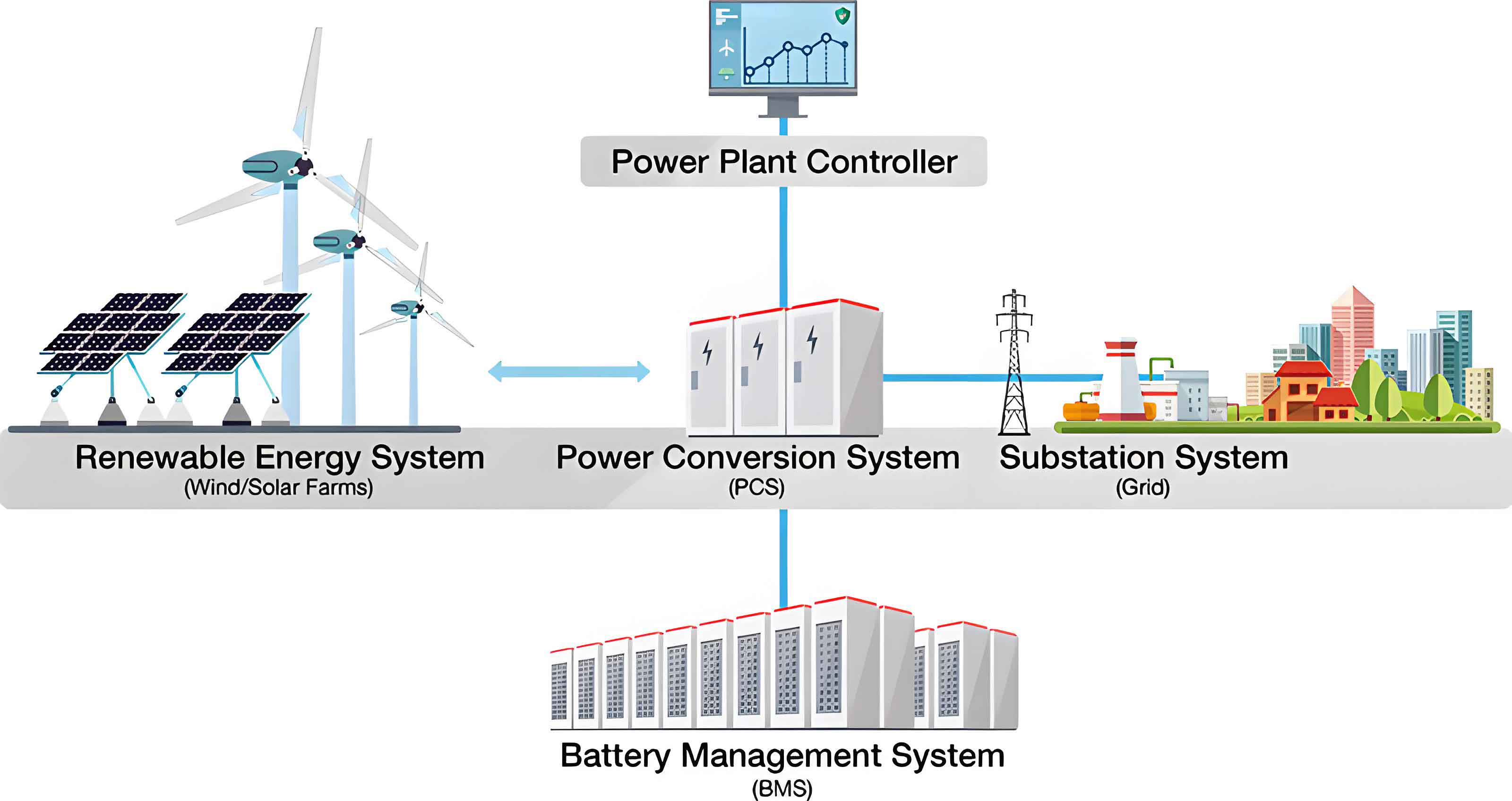
The overall structure of the wind-solar complementary power generation hydrogen storage system is illustrated in the system flowchart. The main components include a wind turbine generator, a photovoltaic (PV) array, a lithium-ion battery pack, an alkaline electrolyzer, a proton exchange membrane fuel cell (PEMFC), power converters, and a hydrogen storage tank. In this off-grid configuration, the wind and solar power are combined on a common DC bus through DC/DC and AC/DC converters. The energy storage system is connected to the same DC bus to absorb power fluctuations and regulate the voltage. The electrolyzer consumes the regulated power to produce hydrogen, which is compressed and stored in a high-pressure tank. When the renewable power is insufficient, the stored hydrogen is supplied to the PEMFC to generate electricity, thus ensuring a continuous power supply to the load. This hybrid configuration enables an efficient utilization of renewable resources while preserving the stability of the energy storage system.
I have established mathematical models for each subsystem in MATLAB/Simulink. The models allow the analysis of dynamic characteristics under various operating conditions. The following subsections describe the modeling approach for each component.
2.1 Wind Power Generation Subsystem
Wind turbines convert the kinetic energy of wind into mechanical power and then into electricity. In this study, I adopt a direct-drive permanent magnet synchronous generator (PMSG) type wind turbine because of its high reliability, efficiency, and low maintenance requirements. The wind speed model is described as a combination of four components: basic wind \(v_A\), gust wind \(v_B\), ramp wind \(v_C\), and random wind \(v_D\). The basic wind is represented by the Weibull distribution:
$$
v_{A}=A\cdot\Gamma\left(1+\frac{1}{k}\right)
$$
where \(A\) is the scale parameter, \(k\) is the shape parameter, and \(\Gamma\) is the gamma function. The gust wind model captures sudden changes in wind speed:
$$
v_B = \begin{cases}
0, & t < T_{1G} \\
v_{Gm}\left(1-\frac{1}{2}\cos\left(2\pi\frac{t-T_{1G}}{T_G}-1\right)\right), & T_{1G}\le t \le T_{1G}+T_G \\
0, & t > T_{1G}+T_G
\end{cases}
$$
The power extracted from the wind is given by:
$$
P = \frac{1}{2}\rho A C_p(\lambda,\beta) v^3
$$
where \(\rho\) is the air density, \(A\) is the rotor swept area, \(v\) is the wind speed, and \(C_p\) is the power coefficient. The power coefficient is a nonlinear function of the tip-speed ratio \(\lambda\) and the blade pitch angle \(\beta\):
$$
C_p(\lambda,\beta) = 0.8\left(0.55\beta -0.003\beta^2 -13\right)\exp\left(-\frac{17.4}{\lambda_i}\right) + 2.19\lambda_i
$$
$$
\frac{1}{\lambda_i} = \frac{1}{\lambda + 0.02\beta} – \frac{0.004}{\beta^3+1}
$$
The tip-speed ratio is defined as \(\lambda = \omega R / v\), where \(\omega\) is the rotor angular speed and \(R\) is the rotor radius. Figure shows the \(C_p-\lambda\) curves for different pitch angles. It is evident that for a fixed pitch angle, there is an optimal tip-speed ratio maximizing \(C_p\). Smaller pitch angles yield higher maximum \(C_p\) values, so pitch angle \(\beta=0\) is preferred for maximum power extraction. The wind turbine output power versus rotor speed is displayed for various wind speeds. The maximum power point tracking (MPPT) adjusts the rotor speed to achieve optimal power output.
The PMSG model in the d-q reference frame can be described by the following voltage equations:
$$
\begin{cases}
u_{sd} = R_s i_{sd} + L_{sd}\frac{di_{sd}}{dt} – \omega_s L_{sq}i_{sq} \\
u_{sq} = R_s i_{sq} + L_{sq}\frac{di_{sq}}{dt} + \omega_s L_{sd}i_{sd} + \omega_s\psi_f
\end{cases}
$$
The electromagnetic torque is given by:
$$
T_e = \frac{3}{2}n_p\left(\psi_f i_{sq} + (L_{sd}-L_{sq})i_{sd}i_{sq}\right)
$$
The active and reactive power outputs from the stator are:
$$
\begin{cases}
P_s = \frac{3}{2}(u_{sd}i_{sd}+u_{sq}i_{sq}) \\
Q_s = \frac{3}{2}(u_{sq}i_{sd}-u_{sd}i_{sq})
\end{cases}
$$
The parameters of the wind turbine used in the simulation are listed in the following table:
| Parameter | Symbol | Value |
|---|---|---|
| Air density (kg/m³) | \(\rho\) | 1.23 |
| Rotor radius (m) | \(R\) | 1.94 |
| Coefficient \(C_1\) | \(C_1\) | 0.793 |
| Coefficient \(C_2\) | \(C_2\) | 117 |
| Coefficient \(C_3\) | \(C_3\) | 0.5 |
| Coefficient \(C_4\) | \(C_4\) | 6 |
2.2 Photovoltaic Generation Subsystem
Photovoltaic cells convert sunlight directly into electricity via the photovoltaic effect. The widely used single-diode model is adopted here. The equivalent circuit consists of a current source, a diode, a series resistance \(R_s\), and a shunt resistance \(R_{sh}\). The output current is expressed as:
$$
I = I_{ph} – I_d – \frac{V+IR_s}{R_{sh}}
$$
where \(I_{ph}\) is the photogenerated current, and \(I_d\) is the diode current given by:
$$
I_d = I_{os}\left[\exp\left(\frac{q(V+IR_s)}{AKT}\right)-1\right]
$$
Here, \(q\) is the electron charge, \(K\) is the Boltzmann constant, \(T\) is the cell temperature, \(A\) is the ideality factor, and \(I_{os}\) is the reverse saturation current. The photogenerated current depends on irradiation and temperature:
$$
I_{ph} = \frac{\lambda}{1000}\left[I_{scr}+K_t(T-298)\right]
$$
where \(\lambda\) is the solar irradiance (W/m²), \(I_{scr}\) is the short-circuit current at standard test conditions, and \(K_t\) is the temperature coefficient. The open-circuit voltage varies with temperature:
$$
V_{oc} = V_{ocs} + K_t(T-298)
$$
The characteristic curves of the PV panel are shown in the simulation results. Figure displays the I-V and P-V curves under constant temperature and varying irradiance. It is observed that the short-circuit current and maximum power increase with irradiance. Under constant irradiance and varying temperature, the open-circuit voltage decreases as temperature rises, while the current slightly increases. The fill factor \(FF\) is defined as:
$$
FF = \frac{P_m}{I_{sc}V_{oc}} = \frac{I_m V_m}{I_{sc}V_{oc}}
$$
The conversion efficiency is \(\eta = P_m/P_{in}\). The parameters used in the PV model are listed below:
| Parameter | Value |
|---|---|
| Short-circuit current \(I_{sc}\) | 9.3 A |
| Maximum power point current \(I_m\) | 8.8 A |
| Open-circuit voltage \(V_{oc}\) | 39.3 V |
| Maximum power point voltage \(V_m\) | 32.4 V |
2.3 Lithium-Ion Battery Energy Storage System
The energy storage system in this work is based on a lithium-ion battery pack. Lithium-ion batteries are preferred because of their high energy density, long cycle life, and high efficiency. A second-order RC equivalent circuit model is used to describe the dynamic behavior of the battery. The model consists of a voltage source \(U_{oc}(SOC)\), internal resistance \(R_0\), and two RC networks (\(R_1C_1\) and \(R_2C_2\)) representing electrochemical polarization and concentration polarization. The state equations are:
$$
\begin{cases}
\frac{dU_1}{dt} = -\frac{U_1}{R_1C_1} + \frac{I_L}{C_1} \\
\frac{dU_2}{dt} = -\frac{U_2}{R_2C_2} + \frac{I_L}{C_2}
\end{cases}
$$
where \(U_1\) and \(U_2\) are the voltages across the RC networks, and \(I_L\) is the load current (positive for discharge, negative for charge). The terminal voltage \(U_L\) is:
$$
U_L = U_{oc}(SOC) – U_1 – U_2 – I_L R_0
$$
The state of charge (SOC) is defined as the remaining capacity percentage:
$$
SOC = \frac{Q}{Q_N}\times 100\%
$$
where \(Q\) is the current remaining capacity and \(Q_N\) is the nominal capacity. The SOC dynamics are governed by the Coulomb counting equation:
$$
SOC(t) = SOC(0) – \frac{1}{Q_N}\int_0^t I_L(\tau) d\tau
$$
For the discrete-time state-space representation, I define the state vector \(x = [SOC, U_1, U_2]^T\). The state transition equation is:
$$
\begin{bmatrix}
SOC(k+1) \\
U_1(k+1) \\
U_2(k+1)
\end{bmatrix}
=
\begin{bmatrix}
1 & 0 & 0 \\
0 & e^{-\Delta t/\tau_1} & 0 \\
0 & 0 & e^{-\Delta t/\tau_2}
\end{bmatrix}
\begin{bmatrix}
SOC(k) \\
U_1(k) \\
U_2(k)
\end{bmatrix}
+
\begin{bmatrix}
-\eta\Delta t/Q_N \\
R_1(1-e^{-\Delta t/\tau_1}) \\
R_2(1-e^{-\Delta t/\tau_2})
\end{bmatrix}
I_L(k)
$$
where \(\tau_1=R_1C_1\), \(\tau_2=R_2C_2\), and \(\eta\) is the Coulombic efficiency. The measurement equation is:
$$
U_L(k) = U_{oc}(SOC(k)) – U_1(k) – U_2(k) – R_0I_L(k)
$$
To accurately estimate SOC, I adopt the unscented Kalman filter (UKF), which is well-suited for nonlinear systems. The performance of the energy storage system relies heavily on the accuracy of SOC estimation, as an incorrect SOC estimate can lead to overcharge or overdischarge, reducing battery life and potentially causing safety hazards.
Table below compares different battery types. In this research, a 20 kW lithium-ion battery pack is used.
| Parameter | Lithium-ion | Lead-acid | NaS | Flow | NiMH |
|---|---|---|---|---|---|
| Specific energy (Wh/kg) | 90-190 | 30-50 | 150-240 | 50-130 | 80-90 |
| Specific power (W/kg) | 150-3300 | 200-315 | 90-230 | 50-140 | 160-230 |
| Round-trip efficiency (%) | 90-95 | 60-75 | 80-90 | 75-85 | 55-65 |
| Cycle life | ~3000 | 500-1000 | 1500-2500 | >16000 | ~2500 |
2.4 Alkaline Electrolyzer
Alkaline water electrolysis is a mature technology for hydrogen production. The electrolyzer consists of an anode, a cathode, a diaphragm, and an alkaline electrolyte (typically KOH). The overall reaction is:
$$
2H_2O \rightarrow 2H_2 + O_2
$$
The anode and cathode half-reactions are:
$$
\text{Anode: } 4OH^- \rightarrow O_2 + 2H_2O + 4e^-
$$
$$
\text{Cathode: } 4H_2O + 4e^- \rightarrow 2H_2 + 4OH^-
$$
The cell voltage of the electrolyzer is composed of the open-circuit voltage (reversible voltage) \(E\), the activation overpotential \(V_{act}\), and the ohmic overpotential \(V_{ohm}\):
$$
V_{el} = E + V_{act} + V_{ohm}
$$
The reversible voltage is given by the Nernst equation:
$$
E = E_0 + \frac{RT}{2F}\ln\left(\frac{p_{H_2}p_{O_2}^{1/2}}{a_{H_2O}}\right)
$$
where \(p_{H_2}\) and \(p_{O_2}\) are the partial pressures of hydrogen and oxygen, and \(a_{H_2O}\) is the water activity. The activation overpotential is:
$$
V_{act} = \frac{RT}{2\alpha F}\ln\left(\frac{i}{i_0}\right)
$$
with \(\alpha\) the transfer coefficient, \(i\) the current density, and \(i_0\) the exchange current density. The ohmic overpotential is:
$$
V_{ohm} = i R_{ohm}
$$
where \(R_{ohm}\) is the ohmic resistance of the electrolyte and membrane. The I-V characteristic of the electrolyzer can be expressed empirically as:
$$
U_{el} = n_c \left[ U_r + \frac{r_1 + r_2 T_{el}}{A} I_{el} + (k_{T1} + k_{T2} T_{el} + k_{T3} T_{el}^2)\ln\left(\frac{k_{el} I_{el}}{A} + 1\right)\right]
$$
The hydrogen production rate is proportional to the current and the current efficiency:
$$
\dot{n}_{H_2} = \eta_F \frac{n_c I_{el}}{zF}
$$
where \(z=2\) is the number of electrons per hydrogen molecule, and \(\eta_F\) is the Faraday efficiency. For an alkaline electrolyzer, the Faraday efficiency is estimated as:
$$
\eta_F = \frac{k_f (I_{el}/A)}{1 + k_f (I_{el}/A)}
$$
In this model, the electrolyzer operates with a maximum power of 70 kW and an optimal power of 50 kW. The parameters used for the electrolyzer simulation are:
| Parameter | Value |
|---|---|
| \(k_r\) (V/K) | 1.91×10⁻³ |
| \(r_1\) (Ω·m²) | 8.182×10⁻⁵ |
| \(r_2\) (Ω·m²/°C) | -4.49×10⁻⁷ |
| \(k_{T1}\) (m²/A) | 2.32×10⁻² |
| \(k_{T2}\) (m²·K/A) | -0.14 |
| \(k_{T3}\) (m²·K²/A) | 1.177×10³ |
| Number of cells \(n_c\) | 1 |
| Electrode area \(A\) (m²) | 0.1 |
| Reversible voltage \(U_r^0\) (V) | 1.21 |
2.5 Proton Exchange Membrane Fuel Cell (PEMFC)
The PEMFC operates in reverse of the electrolyzer, converting hydrogen and oxygen into electricity and water. The reactions are:
$$
\text{Anode: } H_2 \rightarrow 2H^+ + 2e^-
$$
$$
\text{Cathode: } \frac{1}{2}O_2 + 2H^+ + 2e^- \rightarrow H_2O
$$
$$
\text{Overall: } H_2 + \frac{1}{2}O_2 \rightarrow H_2O
$$
The output voltage of a single cell is the reversible voltage minus the activation, ohmic, and concentration losses. The performance curves from the simulation show that increasing the operating temperature improves the cell voltage and power output. The PEMFC is used as a backup generator when the renewable power is insufficient. The parameters for the PEMFC model are provided in the following table:
| Parameter | Value |
|---|---|
| Exchange current density \(I_{fc}\) (mA) | 53.78 |
| Number of cells \(N\) | 25 |
| Anode volume \(V_{an}\) (m³) | 0.005 |
| Cathode volume \(V_{ca}\) (m³) | 0.01 |
| Anode resistance \(R_{acl}\) (Ω) | 8.416 |
| Cathode resistance \(R_{co}\) (Ω) | 8.23 |
| Entropy change \(\Delta S\) (kJ/mol) | -162.1 |
| Gibbs free energy change \(\Delta G\) (kJ/mol) | 274.3 |
| Enthalpy change \(\Delta H\) (kJ/mol) | 287.1 |
2.6 Power Converters and Hydrogen Storage
Power converters are essential for interfacing the various components to the DC bus. Boost converters are used to step up the voltage from the PV panels and fuel cells, while buck or bidirectional converters are used for the battery. The boost converter’s voltage relation is:
$$
V_o = \frac{V_i}{1-D}
$$
where \(D\) is the duty cycle. The hydrogen storage system employs a high-pressure tank. The compressor power is modeled as:
$$
P_{cp} = \frac{1}{\eta_{cp}} c_{p,H2} W_{cp} T_{cp} \left[\left(\frac{P_2}{P_1}\right)^{\frac{\kappa-1}{\kappa}} – 1\right]
$$
where \(c_{p,H2}\) is the specific heat capacity, \(W_{cp}\) is the mass flow rate, and \(\kappa\) is the specific heat ratio. The simulated hydrogen inflow rate and tank pressure are shown in the results.
3. Energy Storage System Characterization and SOC Estimation
3.1 Unscented Kalman Filter (UKF) Overview
The state estimation of the energy storage system is a critical task for optimal power management. The classical Kalman filter is only applicable to linear systems. For nonlinear systems, the extended Kalman filter (EKF) performs a first-order linearization via Taylor expansion, which can introduce large errors for strong nonlinearities. The unscented Kalman filter (UKF) avoids this problem by using the unscented transform (UT) to propagate the mean and covariance through the nonlinear function. UT selects a set of sigma points that capture the true mean and covariance of the state distribution. The UKF algorithm is summarized below.
Consider a nonlinear discrete-time system described by:
$$
\begin{cases}
X(k+1) = f(X(k), W(k)) \\
Z(k) = h(X(k), V(k))
\end{cases}
$$
where \(X(k)\) is the state vector, \(Z(k)\) is the measurement vector, \(W(k)\) is the process noise with covariance \(Q\), and \(V(k)\) is the measurement noise with covariance \(R\). The UKF algorithm consists of the following steps:
Step 1: Initialization
$$
\hat{X}(0) = E[X(0)], \quad P(0) = E[(X(0)-\hat{X}(0))(X(0)-\hat{X}(0))^T]
$$
Step 2: Sigma point generation
For a state dimension \(n\), generate \(2n+1\) sigma points \(\mathcal{X}_i\) and weights \(w_i\):
$$
\mathcal{X}_0 = \bar{X}, \quad w_0^m = \frac{\lambda}{n+\lambda}
$$
$$
\mathcal{X}_i = \bar{X} + \sqrt{(n+\lambda)P}, \quad w_i^m = \frac{1}{2(n+\lambda)}, \quad i=1,\ldots,n
$$
$$
\mathcal{X}_{i+n} = \bar{X} – \sqrt{(n+\lambda)P}, \quad w_i^c = \frac{1}{2(n+\lambda)}, \quad i=n+1,\ldots,2n
$$
where \(\lambda = \alpha^2(n+\kappa)-n\), \(\alpha\) controls the spread of sigma points, and \(\kappa\) is a scaling parameter. The covariance weights \(w_i^c\) include an additional term involving \(\beta\):
$$
w_0^c = \frac{\lambda}{n+\lambda} + (1-\alpha^2+\beta)
$$
Step 3: Prediction
Each sigma point is propagated through the state transition function:
$$
\mathcal{X}_i(k+1|k) = f(\mathcal{X}_i(k|k))
$$
The predicted state mean and covariance are:
$$
\hat{X}(k+1|k) = \sum_{i=0}^{2n} w_i^m \mathcal{X}_i(k+1|k)
$$
$$
P(k+1|k) = \sum_{i=0}^{2n} w_i^c \left[\mathcal{X}_i(k+1|k)-\hat{X}(k+1|k)\right]\left[\mathcal{X}_i(k+1|k)-\hat{X}(k+1|k)\right]^T + Q
$$
Step 4: Measurement update
The sigma points are transformed through the measurement function:
$$
\mathcal{Z}_i(k+1|k) = h(\mathcal{X}_i(k+1|k))
$$
The predicted measurement mean, innovation covariance, and cross-covariance are:
$$
\hat{Z}(k+1|k) = \sum_{i=0}^{2n} w_i^m \mathcal{Z}_i(k+1|k)
$$
$$
P_{ZZ} = \sum_{i=0}^{2n} w_i^c \left[\mathcal{Z}_i(k+1|k)-\hat{Z}(k+1|k)\right]\left[\mathcal{Z}_i(k+1|k)-\hat{Z}(k+1|k)\right]^T + R
$$
$$
P_{XZ} = \sum_{i=0}^{2n} w_i^c \left[\mathcal{X}_i(k+1|k)-\hat{X}(k+1|k)\right]\left[\mathcal{Z}_i(k+1|k)-\hat{Z}(k+1|k)\right]^T
$$
The Kalman gain is computed as:
$$
K = P_{XZ}P_{ZZ}^{-1}
$$
The state and covariance are updated:
$$
\hat{X}(k+1|k+1) = \hat{X}(k+1|k) + K\left[Z(k+1)-\hat{Z}(k+1|k)\right]
$$
$$
P(k+1|k+1) = P(k+1|k) – K P_{ZZ} K^T
$$
The UKF provides more accurate state estimates than EKF for nonlinear systems and avoids calculating Jacobian matrices. In the comparison test, UKF outperforms EKF in tracking performance, with an error reduction of more than 30% in some cases.
3.2 SOC Estimation Using UKF
For the battery energy storage system, the state vector is \(X = [SOC, U_1, U_2]^T\). The nonlinear measurement equation involves the open-circuit voltage \(U_{oc}(SOC)\), which is a nonlinear function of SOC. In this work, the SOC-OCV relationship is obtained from experimental data and approximated by a polynomial. The UKF algorithm estimates SOC recursively, using the measured terminal voltage and current. Figure shows the SOC estimation result using UKF under a constant current discharge. The estimated SOC closely tracks the true SOC, with the estimation error remaining within 0.3%. The comparison between UKF and EKF in SOC estimation confirms the superiority of UKF, as the UKF converges faster and provides smoother estimates.
The accurate SOC estimation is vital for the stable operation of the energy storage system. In the proposed fuzzy control strategy, the estimated SOC is used as an input to the fuzzy logic controller, which adjusts the charging/discharging power reference. If the SOC deviates from its normal operating range, the controller modifies the power reference to restore the SOC to a safe level, thereby preventing overcharge and overdischarge.
3.3 Parameter Identification Using Recursive Least Squares
The accuracy of the battery model depends on the values of \(R_0\), \(R_1\), \(C_1\), \(R_2\), and \(C_2\). These parameters vary with temperature, SOC, and current. To obtain reliable model parameters for the SOC estimator, I apply the recursive least squares (RLS) algorithm for online parameter identification. The transfer function of the second-order RC model in the frequency domain is:
$$
G(s) = \frac{U_{oc}(s)-U_L(s)}{I_L(s)} = -R_0 – \frac{R_1}{1+R_1C_1s} – \frac{R_2}{1+R_2C_2s}
$$
Using bilinear transformation, the discrete-time transfer function can be expressed as a linear regression model:
$$
y(k) = \phi^T(k)\theta + v(k)
$$
where \(y(k)\) is the terminal voltage, \(\phi(k)\) contains the historical input/output data, and \(\theta\) is the parameter vector to be identified. The RLS algorithm updates the parameter estimate \(\hat{\theta}\) recursively:
$$
\hat{\theta}(k) = \hat{\theta}(k-1) + L(k)\left[y(k)-\phi^T(k)\hat{\theta}(k-1)\right]
$$
$$
L(k) = \frac{P(k-1)\phi(k)}{1+\phi^T(k)P(k-1)\phi(k)}
$$
$$
P(k) = \left[I – L(k)\phi^T(k)\right]P(k-1)
$$
The parameter identification process is shown in the simulation. With accurate parameter identification, the SOC estimation becomes more robust under varying operating conditions.
4. Power Regulation Based on Fuzzy UKF
4.1 Overall Control Strategy
The proposed control strategy integrates the UKF-based SOC estimation with a fuzzy logic controller to regulate the power flow of the energy storage system. The schematic diagram of the control structure is shown in the previous figure. The wind-solar power is first smoothed by a UKF filter to reduce high-frequency fluctuations. The smoothed power is then supplied to the battery energy storage system, which acts as a buffer. The UKF observer estimates the battery SOC and feeds it to the fuzzy controller. The fuzzy controller adjusts the battery power command \(P_b^*\) based on the SOC error and the power imbalance. The adjusted power ensures that the SOC remains within the desired range, while simultaneously maintaining a stable power output to the electrolyzer.
4.2 Fuzzy Logic Control Theory
Fuzzy logic control is a model-free control method that mimics human reasoning. It transforms expert knowledge into linguistic rules and is particularly effective for complex, nonlinear, and uncertain systems. The fuzzy controller in this work has two inputs: the SOC error \(e_{SOC} = SOC – SOC_{ref}\) and the battery power \(P_b\), or equivalently the smoothing factor. The output is the fuzzy adjustment coefficient \(m\). The battery power command is modified as:
$$
P_b = P_{b0} + K_m \cdot m
$$
where \(P_{b0}\) is the base power command from the smoothing filter and \(K_m\) is a scaling factor. Alternatively, the fuzzy controller can adjust the filter parameter to change the smoothing intensity. When the SOC is too high, the controller reduces the charging power or increases the discharging power; when the SOC is too low, the controller increases charging or reduces discharging. In extreme cases, the controller stops the power flow to protect the battery.
4.3 Fuzzy Rules for SOC Stabilization
I design a set of fuzzy rules based on the operational requirements of the energy storage system. The inputs are the SOC level (measured by the estimated SOC) and its derivative. The output is the power adjustment factor \(m\). The linguistic variables for SOC are defined as {PL (Positive Large), PH (Positive High), O (Optimal), NL (Negative Low), NH (Negative High)}. The rule table is as follows:
| \(m\) | PB | PS | ZO | NS | NB |
|---|---|---|---|---|---|
| PH | 1.05 | 1.01 | 1 | 0.09 | 0.03 |
| PL | 1.03 | 1.02 | 1 | 0.07 | 0.06 |
| O | 0.8 | 0.9 | 1 | 0.09 | 0.08 |
| NL | 0.07 | 0.06 | 1 | 1.04 | 1.05 |
| NH | 0.03 | 0.05 | 1 | 1.03 | 1.07 |
Here, PB, PS, ZO, NS, NB are the fuzzy sets for the battery power error, while PH, PL, O, NL, NH represent the SOC linguistic categories. The membership functions are chosen as triangular and Gaussian functions, as displayed in the simulation. The fuzzy surface plot shows the relationship between the inputs and the output \(m\).
To ensure the electrolyzer continues to operate within acceptable limits, I define several operational scenarios based on the SOC condition and the electrolyzer power constraints:
| Scenario | SOC Condition | Electrolyzer Power |
|---|---|---|
| 1 | SOC in normal range | \(P_{EL}=P_{opt}\) |
| 2 | SOC low, \(P_{in} > P_{EL}^{min}\) | \(P_{EL}=P_{EL}^{min}\) |
| 3 | SOC low, \(P_{in} \le P_{EL}^{min}\) | \(P_{EL}=P_{EL}^{min}\) or stop |
| 4 | SOC high, \(P_{in} < P_{EL}^{max}\) | \(P_{EL}=P_{EL}^{max}\) |
| 5 | SOC high, \(P_{in} \ge P_{EL}^{max}\) | \(P_{EL}=P_{EL}^{max}\) |
These scenarios ensure that when the battery SOC is partially high or low, the power supplied to the electrolyzer is adjusted to either the minimum or maximum allowable value, so that the battery can recover its SOC without sacrificing the stability of the overall system.
5. Simulation Results and Discussion
The wind-solar complementary hydrogen production system with the proposed fuzzy UKF controller is implemented in MATLAB/Simulink. Real measured data from a wind farm and a photovoltaic plant are used as inputs to the simulation. The system parameters are listed in the following table:
| Parameter | Value |
|---|---|
| Maximum SOC (SOC_max) | 0.95 |
| Minimum SOC (SOC_min) | 0.05 |
| Battery rated power | 20 kW |
| Maximum load power | 125 kW |
| Maximum electrolyzer power | 70 kW |
| Optimal electrolyzer power | 50 kW |
| Maximum PEMFC power | 85 kW |
| Optimal PEMFC power | 65 kW |
First, I verify the SOC regulation capability of the fuzzy controller. Two extreme initial SOC values are considered: SOC = 90% (high) and SOC = 10% (low). The simulation results are shown in the figures. In the high-SOC case, without any control, the SOC remains high, which risks overcharging. With the fuzzy control, the SOC gradually decreases to around 70% within 27 hours, as the controller reduces the charging power and increases the discharging power. Similarly, in the low-SOC case, the fuzzy control increases the charging power and reduces the discharging power, allowing the SOC to recover to over 30% in about 26 hours. In contrast, without control, the SOC remains at a low level, potentially leading to overdischarge.
The wind and solar power outputs used in the simulation are shown in the figures. The total complementary power has lower fluctuation than either source individually. The load power profile is also illustrated. The net power that flows into the energy storage system is the difference between the renewable power and the load power. The UKF-smoothed power is used as the base power command for the battery.
Figure presents the SOC estimation result using the UKF. The estimated SOC closely follows the true SOC, with a small error bound of 0.3%. The battery output power under fuzzy control is shown in the figure. It can be observed that when the SOC drops below the setpoint, the controller reduces the discharge power (or increases the charge power) to restore the SOC. The fuzzy-controlled SOC is displayed in the figure, where the SOC is maintained between 0.2 and 0.8, within the designated safe range.
Finally, the electrolyzer output power is illustrated in the figure. During the simulation, the electrolyzer operates at different power levels depending on the SOC condition and the available power. As shown, the electrolyzer runs at the maximum power of 70 kW during periods when surplus power is high and the SOC is within acceptable limits, at the minimum power of 35 kW when SOC needs to recover, and at the optimal power of 50 kW during normal operation. The controller effectively reduces the number of on/off cycles of the electrolyzer and ensures a smoother hydrogen production process. The overall system stability is significantly improved, with the DC bus voltage maintained at a nearly constant level.
To further demonstrate the superiority of the proposed fuzzy UKF strategy, I compare it with a conventional EKF-based SOC estimation and a fixed power control method. The results confirm that the proposed method provides more accurate SOC estimation and more robust power regulation, leading to a more stable hydrogen production rate.
6. Conclusion
This thesis has presented a comprehensive study on the stability of a wind-solar complementary power generation system with an integrated hydrogen energy storage system. The energy storage system, composed of a lithium-ion battery pack and an alkaline electrolyzer, plays a central role in smoothing the intermittent renewable power and delivering stable hydrogen output. The following conclusions can be drawn from this work:
(1) The established mathematical models for each subsystem accurately describe their steady-state and dynamic behavior. The wind turbine model effectively captures the nonlinear relationship between wind speed and power output, while the photovoltaic model reflects the influence of irradiance and temperature. The battery model with a second-order RC network provides a good balance between accuracy and computational efficiency.
(2) The unscented Kalman filter is an effective tool for SOC estimation in the energy storage system. Compared with the extended Kalman filter, the UKF yields higher estimation accuracy and better convergence properties, especially under strong nonlinear conditions. The recursive least squares-based parameter identification further improves the model fidelity.
(3) The proposed fuzzy UKF control strategy successfully maintains the battery SOC within its safe operating range. By automatically adjusting the charging/discharging power based on the estimated SOC, the controller prevents overcharge and overdischarge while ensuring a continuous and stable power supply to the electrolyzer. The simulation results demonstrate that the electrolyzer output power is maintained at a stable level, with reduced fluctuations and fewer shutdowns.
(4) The integration of the battery energy storage system with hydrogen production not only enhances the system flexibility but also increases the overall energy utilization efficiency. The proposed control scheme is suitable for off-grid renewable hydrogen production systems and can be extended to grid-connected applications in the future.
Future research could focus on the full modeling of all components, including power electronics and auxiliary devices, and on exploring the grid-connected operation mode. Furthermore, more advanced parameter identification techniques and intelligent control algorithms, such as model predictive control or deep reinforcement learning, could be integrated to further improve the performance of the energy storage system. The economic viability and long-term degradation of the battery and electrolyzer should also be considered in practical implementations.
In summary, this thesis provides a solid theoretical foundation and a practical control framework for the stable operation of wind-solar complementary hydrogen production systems, demonstrating the pivotal role of an advanced energy storage system in enabling a sustainable and reliable renewable energy future.