
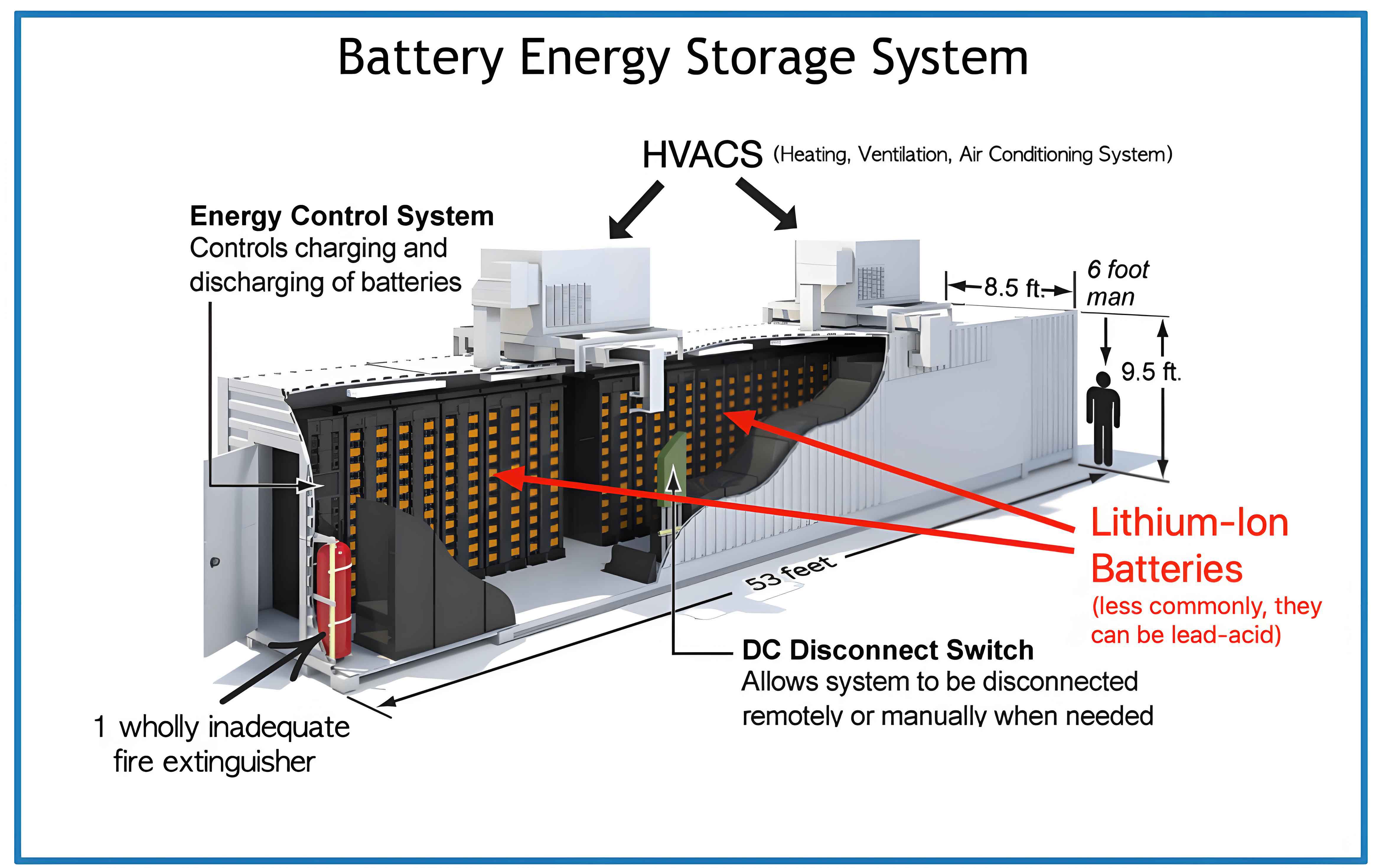
In the context of the global energy transition, the penetration of renewable energy sources such as photovoltaic and wind power has been increasing rapidly. The intermittency and uncertainty of these sources, combined with the fact that most renewable generators are connected to the grid through power electronic converters, cause a significant reduction in the overall system inertia and damping. Consequently, frequency and voltage stability of the power grid face severe challenges. In order to address these issues, the virtual synchronous generator (VSG) technique has been proposed, which mimics the electromechanical characteristics of a conventional synchronous generator within a power electronic converter. By embedding the VSG control algorithm into an energy storage system, the converter can provide virtual inertia and damping to the grid, thereby supporting frequency and voltage regulation. The work presented in this thesis focuses on control strategies and parameter optimization of VSG-based energy storage systems, studied at both the unit level and the plant level. In particular, I investigate fixed-parameter VSG, adaptive inertia and damping control, multi-mode switching control, and coordinated parallel operation of multiple VSG units.
The core contribution of this thesis is to demonstrate how the energy storage system with VSG control can act as a grid-forming source, improving the resilience of high-renewable power systems. I first develop an accurate simulation model of a photovoltaic plant combined with a battery energy storage system using the VSG controller, and validate its effectiveness under different disturbances. Then, I propose an adaptive optimization strategy for the virtual inertia and damping coefficients, which significantly reduces frequency oscillations and improves dynamic response. Finally, I extend the analysis to a multi-machine parallel configuration and propose a coordination scheme based on particle swarm optimization and dynamic virtual impedance. The simulation results confirm that the proposed methods can effectively suppress power oscillations, reduce frequency deviations, and enhance the overall stability of the system. Throughout the thesis, the term energy storage system appears frequently because the VSG technique relies on the controllable active power exchanged with the storage device.
1. Fundamentals of Synchronous Generators and VSG Control
To emulate the behavior of a conventional synchronous machine, one must first understand its mathematical description. The rotor motion of a synchronous generator is governed by the swing equation, which is written as
$$ J \frac{d\omega}{dt} = T_m – T_e – D_p(\omega – \omega_0) \tag{1} $$
where \(J\) is the moment of inertia, \(\omega\) is the rotor angular velocity, \(\omega_0\) is the nominal angular velocity, \(T_m\) and \(T_e\) are the mechanical torque and electromagnetic torque, respectively, and \(D_p\) is the damping coefficient. The electromagnetic torque can be expressed in terms of the air-gap flux and stator currents, but from a control perspective the important feature is that the inertia provides kinetic energy exchange during transients, while damping contributes to oscillation decay.
In a voltage-source converter, the inertia and damping are not physical properties. However, they can be synthesized through the control algorithm. The VSG control strategy implemented in this thesis uses the following active-power frequency loop:
$$ P_m = P_{ref} + k_p(\omega_0 – \omega) \tag{2} $$
$$ J \frac{d\omega}{dt} = \frac{P_m – P_e}{\omega_0} – D(\omega – \omega_0) \tag{3} $$
$$ \frac{d\theta}{dt} = \omega \tag{4} $$
Here, \(P_{ref}\) is the active power reference, \(P_e\) is the measured output active power, \(k_p\) is the primary frequency droop coefficient, \(D\) is the virtual damping coefficient, \(J\) is the virtual inertia coefficient, and \(\theta\) is the phase angle of the internal voltage. The reactive-power voltage control loop is given by
$$ E = U_{ref} + d_q(U_{ref} – U) + k_q(Q_{ref} – Q) \tag{5} $$
where \(E\) is the magnitude of the internal voltage, \(U\) is the terminal voltage, \(U_{ref}\) is the reference voltage, \(Q\) is the measured reactive power, \(Q_{ref}\) is the reactive power reference, and \(k_q\), \(d_q\) are the corresponding droop and voltage regulation coefficients. Equations (2)–(5) form the basis of the voltage-source VSG controller, which generates the reference voltage amplitude and phase for the inner current and voltage control loops.
In my research, I first implemented this basic VSG controller in an energy storage system connected to a 100 MW photovoltaic power plant. The system model was built in DIgSILENT/PowerFactory. The storage capacity was varied from 10% to 50% of the nominal plant capacity. The simulation scenarios included a sudden drop in PV generation, a short-circuit on the transmission line, and a load step change. The results showed that the VSG-controlled energy storage system can effectively support the bus frequency and voltage. For instance, when the PV output dropped abruptly, the frequency decreased to around 49.72 Hz before recovering to 49.76 Hz with a 30% storage capacity. When the storage capacity was increased to 50%, the minimum frequency was only 49.81 Hz, and the recovery time was shorter. This confirms that a larger energy storage system provides stronger inertia support and improves the dynamic performance of the grid.
2. Small-Signal Analysis and Fixed-Parameter Limitations
The basic VSG controller uses fixed values of \(J\) and \(D\). Although the system is stable, the fixed parameters cannot adapt to different operating conditions. To illustrate this, I derived the small-signal model of the VSG connected to a stiff grid. The closed-loop transfer function from active power reference to output active power is
$$ \frac{P_e}{P_{ref}}(s) = \frac{k_p}{\tau s^2 + (D + k_p) s + k_p \tau} \tag{6} $$
where \(\tau = J \omega_0\). The natural angular frequency and damping ratio are
$$ \omega_n = \sqrt{\frac{k_p}{\tau}} \tag{7} $$
$$ \zeta = \frac{D + k_p}{2 \sqrt{k_p \tau}} \tag{8} $$
From (7) and (8), one can see that increasing the virtual inertia \(J\) lowers the damping ratio and increases the settling time, whereas increasing the virtual damping \(D\) improves the damping ratio at the expense of a slower frequency droop response. The fixed-parameter VSG exhibits a trade-off between overshoot and response speed that cannot be optimal for all disturbances.
Table 1 summarizes the dynamic performance of the VSG with different fixed \(J\) and \(D\) values, obtained from time-domain simulations in MATLAB/Simulink. The load step was 15 kW, and the VSG was rated at 15 kW.
| Control Case | \(J\) (kg·m²) | \(D\) (N·m·s/rad) | Overshoot (%) | Settling time (s) | Max frequency deviation (Hz) |
|---|---|---|---|---|---|
| Case 1 (fixed D, varied J) | 0.8 | 10 | 31.3 | 1.2 | 0.42 |
| Case 2 | 1.2 | 10 | 38.8 | 1.6 | 0.46 |
| Case 3 | 1.6 | 10 | 45.0 | 2.0 | 0.50 |
| Case 4 | 2.0 | 10 | 48.8 | >2.0 | 0.53 |
| Case 5 (fixed J=1.2, varied D) | 1.2 | 5 | 63.8 | >2.0 | 0.62 |
| Case 6 | 1.2 | 8 | 42.5 | 2.0 | 0.48 |
| Case 7 | 1.2 | 11 | 35.0 | 1.5 | 0.44 |
| Case 8 | 1.2 | 14 | 25.0 | 1.2 | 0.40 |
Table 1: Dynamic response of VSG with different fixed parameters.
The results clearly show that neither increasing \(J\) nor increasing \(D\) alone can simultaneously reduce both the overshoot and the settling time. Therefore, an adaptive parameter optimization strategy is required, which is presented in the next section.
3. Adaptive Inertia and Damping Optimization for Unit-Level Energy Storage System
In this section, I propose an adaptive control strategy that adjusts the virtual inertia \(J\) and damping \(D\) in real time according to the frequency deviation and its rate of change. The principle is based on the energy exchange in an oscillation cycle. Consider the power angle and rotor frequency curves shown in Figure 1. The whole oscillation process can be divided into four stages, as summarized in Table 2.
| Stage | \(\Delta \omega\) | \(d\omega/dt\) | Behavior | \(J\) adjustment | \(D\) adjustment |
|---|---|---|---|---|---|
| 1 | >0 | >0 | Acceleration | Increase | Increase |
| 2 | <0 | >0 | Deceleration | Decrease | Decrease |
| 3 | <0 | <0 | Acceleration | Increase | Increase |
| 4 | >0 | <0 | Deceleration | Decrease | Decrease |
Table 2: Parameter adjustment rules in different oscillation stages.
Based on the table, I define the adaptive control functions as follows:
$$ J = \begin{cases} J_0, & \left| \frac{d\omega}{dt} \right| \leq C_j \\ J_0 + K_j \left| \frac{d\omega}{dt} \right|, & \left| \frac{d\omega}{dt} \right| > C_j \end{cases} \tag{9} $$
$$ D = \begin{cases} D_0, & |\Delta \omega| \leq C_d \\ D_0 + K_d |\Delta \omega|, & |\Delta \omega| > C_d \end{cases} \tag{10} $$
where \(J_0\) and \(D_0\) are the base values, \(K_j\) and \(K_d\) are the tuning gains, and \(C_j\), \(C_d\) are the thresholds that prevent excessive frequent parameter changes. This adaptive law ensures that the virtual inertia is large when the frequency is accelerating away from the nominal value, and small when the frequency is returning, which speeds up the restoration. Meanwhile, the damping is increased when the frequency deviation is large, helping to limit the overshoot.
To select the optimal parameters \(J_0\), \(D_0\), \(K_j\), \(K_d\), I formulated an optimization problem. The objective is to minimize both the frequency deviation and its rate of change during transients. The problem can be written as
$$ \min \left[ w_1 |\Delta \omega| + w_2 \left| \frac{d\omega}{dt} \right| \right] \tag{11} $$
subject to the following constraints:
$$ J \leq \frac{P_{max}}{\omega_0 \left| \frac{d\omega}{dt} \right|_{max}} \qquad \text{(inertia limit)} \tag{12} $$
$$ D \geq \frac{P_{max} – P_{min}}{\omega_0 (\omega_{max} – \omega_{min})} – k_p \qquad \text{(damping limit)} \tag{13} $$
Equation (12) ensures that the maximum rate of change of frequency does not exceed a prescribed bound, and Equation (13) guarantees that the frequency remains within the allowed range. The Chinese standard GB/T 15945-1995 allows a frequency deviation of ±0.2 Hz for large power systems, and I used this as a reference.
I simulated the proposed adaptive control strategy under a load step of 15 kW. Four cases were compared:
- Case A: \(J\) and \(D\) both adaptive (proposed)
- Case B: \(J\) and \(D\) both fixed
- Case C: \(J\) adaptive, \(D\) fixed
- Case D: \(J\) fixed, \(D\) adaptive
The simulation results are summarized in Table 3. The proposed method (Case A) yields the smallest overshoot and the shortest settling time. The maximum frequency deviation is only 0.2 Hz, compared with 0.5 Hz for the fixed parameter case.
| Case | Active power overshoot (%) | Settling time (s) | Max frequency deviation (Hz) |
|---|---|---|---|
| A (adaptive J&D) | 1.3 | 0.75 | 0.20 |
| B (fixed J&D) | 12.7 | 0.95 | 0.50 |
| C (adaptive J, fixed D) | 7.3 | 0.85 | 0.33 |
| D (fixed J, adaptive D) | 3.6 | 0.80 | 0.28 |
Table 3: Comparison of fixed and adaptive parameter control.
The time-domain waveforms are shown in Figure 12 (not reproduced here). The adaptive control successfully reduces the frequency oscillation and improves the response speed. The virtual inertia and damping coefficients change dynamically with the frequency trajectory, providing the energy storage system with the ability to act like a synchronous generator with adjustable rotor inertia.
3.1 Multi-Mode Switching Control
In normal steady-state operation, the VSG control introduces additional time delay due to its virtual inertia. In contrast, the conventional PQ control offers much faster power tracking. To combine the advantages of both, I designed a multi-mode switching strategy. Under normal conditions, the energy storage converter operates in PQ mode. When a disturbance or fault is detected, the controller switches to VSG mode to provide frequency and voltage support. The switching logic is shown in Figure 13 and implemented as follows:
For the transition from VSG to PQ, the current commands of the PQ mode are initialized to the current values of the VSG mode and then ramped smoothly using a soft-start integrator:
$$ i_{Ld}^* = i_{Ld,c}^* + \int_0^T \Delta i_{Ld} \, dt \tag{14} $$
where \(T\) is the soft-start time and \(\Delta i_{Ld}\) is the step size. This prevents current spikes during the transition. For the transition from PQ to VSG, the VSG output voltage phase tracks the grid phase, ensuring a smooth switch. I have validated the multi-mode switching strategy in MATLAB/Simulink. The results show that the grid-side current and active power remain almost unchanged during the switching instants; only a negligible transient of less than 2 V and no appreciable oscillation appears.
4. Plant-Level Parallel Control of Multi-VSG Energy Storage Systems
For large-scale renewable power plants, a single energy storage converter often cannot meet the required capacity. Multiple VSG units operating in parallel provide a scalable solution. However, parallel operation introduces new stability issues such as power oscillations among the converters. In this section, I study the parallel control of multiple VSG units based on energy storage systems.
4.1 Modeling of Two Parallel VSGs
Figure 1 illustrates the topology of two VSGs connected to a common AC bus. Each VSG has its own LC filter and connecting line impedance. The load is shared between the two units. The power-angle relationship for each VSG when the line impedance is dominantly inductive can be simplified as
$$ P_i = \frac{U_{dc} U_L}{X_i} \sin \theta_i \approx \frac{U_{dc} U_L}{X_i} \theta_i \tag{15} $$
$$ Q_i = \frac{U_L (E_i – U_L)}{X_i} \tag{16} $$
where \(i=1,2\), \(U_{dc}\) is the common DC voltage, \(U_L\) is the load voltage amplitude, \(X_i\) is the equivalent output reactance, and \(\theta_i\) is the power angle.
Combining the swing equation of each VSG with the power-angle relation, I derived the state-space model of the parallel system. The state variables are chosen as the frequency deviations of the two VSGs, the derivative of the first frequency deviation, and the power-angle difference. The linearized model can be written in the form
$$ \dot{x} = A x + B p_L \tag{17} $$
$$ y = C x + D p_L \tag{18} $$
where \(x = [\Delta \omega_1, \Delta \dot{\omega}_1, \Delta \omega_2, \Delta \dot{\omega}_2, \Delta \delta]^T\) and \(p_L\) is the load power disturbance. The matrices \(A\), \(B\), \(C\), and \(D\) are given by the expressions in Section 4.2 of the original thesis. The analysis shows that the eigenvalues of matrix \(A\) depend on the virtual inertias \(J_1, J_2\), damping coefficients \(D_1, D_2\), and droop coefficients \(k_{p1}, k_{p2}\). If the parameters of the two VSGs are not properly coordinated, the system can exhibit weakly damped or even unstable modes.
4.2 Cause of Power Oscillations
To illustrate the influence of parameter differences, I simulated the response of two parallel VSGs to a load step. Figure 14 shows the frequency waveforms when only virtual inertia is present (damping set to zero). When the two VSGs have equal inertia, the frequencies overlap and no oscillation occurs. However, when \(J_1 \neq J_2\), the two frequencies diverge temporarily, causing a power oscillation. Similarly, Figure 15 shows that unequal damping coefficients also lead to frequency separation and power oscillation. The root cause is that different converters have different transient responses, and the lack of coordination makes them fight each other.
4.3 Dynamic Virtual Impedance for Power Decoupling
In order to overcome the coupling between active and reactive power caused by line resistance, I introduced a dynamic virtual impedance in the control loop. The virtual impedance is designed to make the output impedance of the converter appear predominantly inductive, which helps decouple \(P\) from \(U\) and \(Q\) from \(\theta\). The dynamic adjustment law is formulated as
$$ Z_v = \begin{cases} R_n + sL_m, & m \leq 1 \\[6pt] R_n + sL_m + K \int (m Q_1 – Q_2) dt, & m > 1 \end{cases} \tag{19} $$
where \(m = Q_1/Q_2\) is the reactive power sharing ratio, \(R_n\) is a negative virtual resistance that partially cancels the actual resistance, \(L_m\) is the virtual inductance, and \(K\) is the adjustment gain. The negative resistance is slightly lower in absolute value than the actual line resistance, so the overall impedance remains weakly positive and avoids instability. By dynamically adjusting the virtual impedance, the reactive power sharing is improved and the voltage drops are reduced.
4.4 Particle Swarm Optimization for Parallel VSG Parameters
In addition to the virtual impedance, I applied the particle swarm optimization (PSO) algorithm to tune the virtual inertia and damping of each VSG unit. The objective function is designed to minimize the frequency deviation and to achieve a damping ratio close to 0.707, which is the optimal trade-off between overshoot and settling time. The fitness function is defined as
$$ F = 0.5 f_1 + 0.5 f_2 \tag{20} $$
$$ f_1 = \int_0^{T_s} |\Delta \omega| \, dt \tag{21} $$
$$ f_2 = \left| \zeta – 0.707 \right| \tag{22} $$
where \(T_s\) is the simulation time, \(\Delta \omega\) is the frequency deviation in per unit, and \(\zeta\) is the damping ratio estimated from the small-signal model.
The optimization constraints are
$$ \begin{cases} J_{\min 1} \leq J_1 \leq J_{\max 1} \\ J_{\min 2} \leq J_2 \leq J_{\max 2} \\ D_{\min 1} \leq D_1 \leq D_{\max 1} \\ D_{\min 2} \leq D_2 \leq D_{\max 2} \end{cases} \tag{23} $$
The PSO algorithm was run for 300 iterations. The convergence curve is shown in Figure 16. The optimal parameters obtained were \(J_1 = 1.5 \,\text{kg·m}^2\), \(J_2 = 0.8 \,\text{kg·m}^2\), \(D_1 = 5 \,\text{N·m·s/rad}\), and \(D_2 = 23 \,\text{N·m·s/rad}\). These values are different from each other, which indicates that the optimization accounts for the different line impedances or ratings of the two units.
4.5 Simulation Results for Parallel Systems
I built a two-unit VSG parallel model in MATLAB/Simulink. The load step was applied at \(t = 1.5 \text{s}\) and removed at \(t = 3 \text{s}\). The active power responses before and after optimization are shown in Figures 17 and 18, respectively. Before optimization, both VSGs exhibit noticeable power oscillations that decay slowly. After optimization, the oscillations are damped out within 0.2 s, and the steady-state power division is accurate.
The frequency responses are compared in Figures 19 and 20. The optimized system has a maximum frequency deviation of only 0.4 Hz, compared with more than 1 Hz for the non-optimized system. Moreover, the frequency reaches steady state in about 0.3 s after the load change, whereas the non-optimized system requires more than 1 s.
To verify the scalability of the proposed method, I also built a three-unit parallel VSG system using the same optimization procedure. The simulation results are summarized in Table 4. The optimized control effectively suppresses power oscillations and improves the frequency dynamics in a similar manner.
| System | Metric | Before optimization | After optimization |
|---|---|---|---|
| Two VSGs | Max active power overshoot (kW) | 18 | 3 |
| Two VSGs | Settling time after load step (s) | 2.0 | 0.5 |
| Two VSGs | Max frequency deviation (Hz) | 1.5 | 0.35 |
| Three VSGs | Max active power overshoot (kW) | 22 | 5 |
| Three VSGs | Settling time after load step (s) | 2.3 | 0.7 |
| Three VSGs | Max frequency deviation (Hz) | 1.8 | 0.4 |
Table 4: Performance comparison of parallel VSG systems before and after optimization.
The results demonstrate that the proposed parallel optimization control, combining PSO-based parameter tuning and dynamic virtual impedance, is effective for both two-machine and three-machine configurations. The method can be extended to a larger number of units, making it suitable for the coordinated control of a plant-level energy storage system.
5. Conclusion and Future Work
This thesis has investigated the control strategies and parameter optimization of virtual synchronous generators in energy storage systems. The main conclusions are summarized as follows:
- The VSG-controlled energy storage system can provide virtual inertia and damping support to the grid, effectively mitigating frequency and voltage fluctuations caused by renewable power variations, line faults, and load steps. A larger energy storage capacity leads to a higher frequency/voltage nadir and faster recovery.
- Fixed-parameter VSG control exhibits a trade-off between overshoot and settling time. The proposed adaptive inertia and damping adjustment law, which changes the parameters according to the frequency deviation and its rate of change, significantly improves the transient response. The multi-mode switching control realizes a smooth transition between PQ and VSG modes, combining the fast power response with grid-forming support capability.
- In parallel VSG systems, unequal virtual inertias and damping coefficients among the units are the primary cause of power oscillations. The proposed dynamic virtual impedance decouples active and reactive power, while the particle swarm optimization algorithm optimally tunes the control parameters. Simulation results for two and three parallel VSG units confirm that the proposed method effectively suppresses power oscillations, reduces frequency deviations, and shortens the settling time.
There are several aspects that deserve further investigation. First, the storage battery dynamics are not fully modeled in this work; I plan to incorporate a detailed battery model with state-of-charge constraints. Second, more complex parallel phenomena such as circulating currents and harmonic interactions should be studied. Third, for a larger number of VSG units, the communication topology and distributed optimization algorithms should be explored. Finally, hardware-in-the-loop experiments would be valuable to validate the real-time implementation of the proposed strategies. The energy storage system as a flexible resource will play a crucial role in future power grids, and the VSG control plus parameter optimization techniques developed in this thesis contribute to unlocking its full potential.