
1. Introduction
In recent years, driven by the national “Dual Carbon” strategy and the rural revitalization policy, distributed clean energy sources, primarily photovoltaic and wind power, have developed rapidly in rural distribution networks, with the installed capacity of new energy increasing year by year. The rural distribution network will evolve into a local new power system centered on distributed new energy and energy storage, interconnected with the main grid. However, the grid structure of rural distribution networks is weak, and the power supply routes are single, resulting in low power supply quality and voltage levels.
The integration of a high proportion of renewable energy brings changes to the operation mode of rural distribution networks. Due to the difficulty of achieving local consumption, the supply-demand imbalance between source and load is increased, leading to more severe voltage fluctuations in rural distribution networks, with some node voltages even experiencing serious deviations. This is also accompanied by a series of problems such as increased line losses. Therefore, how to achieve full consumption of new energy while ensuring the safe and stable operation of the system has become an urgent problem to be solved in the current construction of new power systems.
Energy storage technology, with its power regulation and energy throughput capabilities, can promote renewable energy consumption and enhance system resilience and safety. Configuring an energy storage system on the distribution network side can effectively smooth new energy fluctuations, alleviate transmission channel congestion, optimize grid power flow, improve voltage stability, and enhance the grid’s frequency regulation and peak shaving capabilities. For the energy storage system itself, only a reasonable construction location and capacity configuration can maximize its role. If the energy storage system is arbitrarily connected to nodes, it may cause voltage fluctuations or even limit violations, increasing line losses and aggravating grid operation pressure. Unreasonable capacity configuration will increase costs and reduce the economy of system operation. Therefore, in rural distribution networks with a high proportion of renewable energy, the reasonable optimization configuration of the energy storage system is an urgent problem to be solved in the construction of distributed and even large-scale energy storage systems.
| Storage Type | Typical Representatives |
|---|---|
| Mechanical energy storage | Pumped hydro storage, compressed air energy storage, flywheel energy storage |
| Electrochemical energy storage | Lead-acid battery, lithium-ion battery, sodium-sulfur battery, flow battery |
| Electrical energy storage | Capacitor energy storage, supercapacitor energy storage |
| Thermal energy storage | Sensible heat storage, thermochemical storage |
| Hydrogen energy storage | Hydrogen storage |
| Storage Type | Compressed Air | Pumped Hydro | Flywheel | Lead-acid | Lithium-ion | Supercapacitor |
|---|---|---|---|---|---|---|
| Power range (MW) | 5~400 | 100~5000 | 0~20 | 0.001~50 | 0.001~0.01 | 0.1~10 |
| Discharge duration | >1~24h | >1~24h | ms~15min | min~h | min~10h | ms~1h |
| Efficiency (%) | 50~89 | 75~85 | 93~95 | 70~90 | 9~98 | 90~95 |
| Lifetime (years) | 20~60 | 40~60 | 400~15 | 5~8 | 5~15 | >20 |
| Cycle times | – | – | >2000 | 300~600 | 100~10000 | >1000000 |
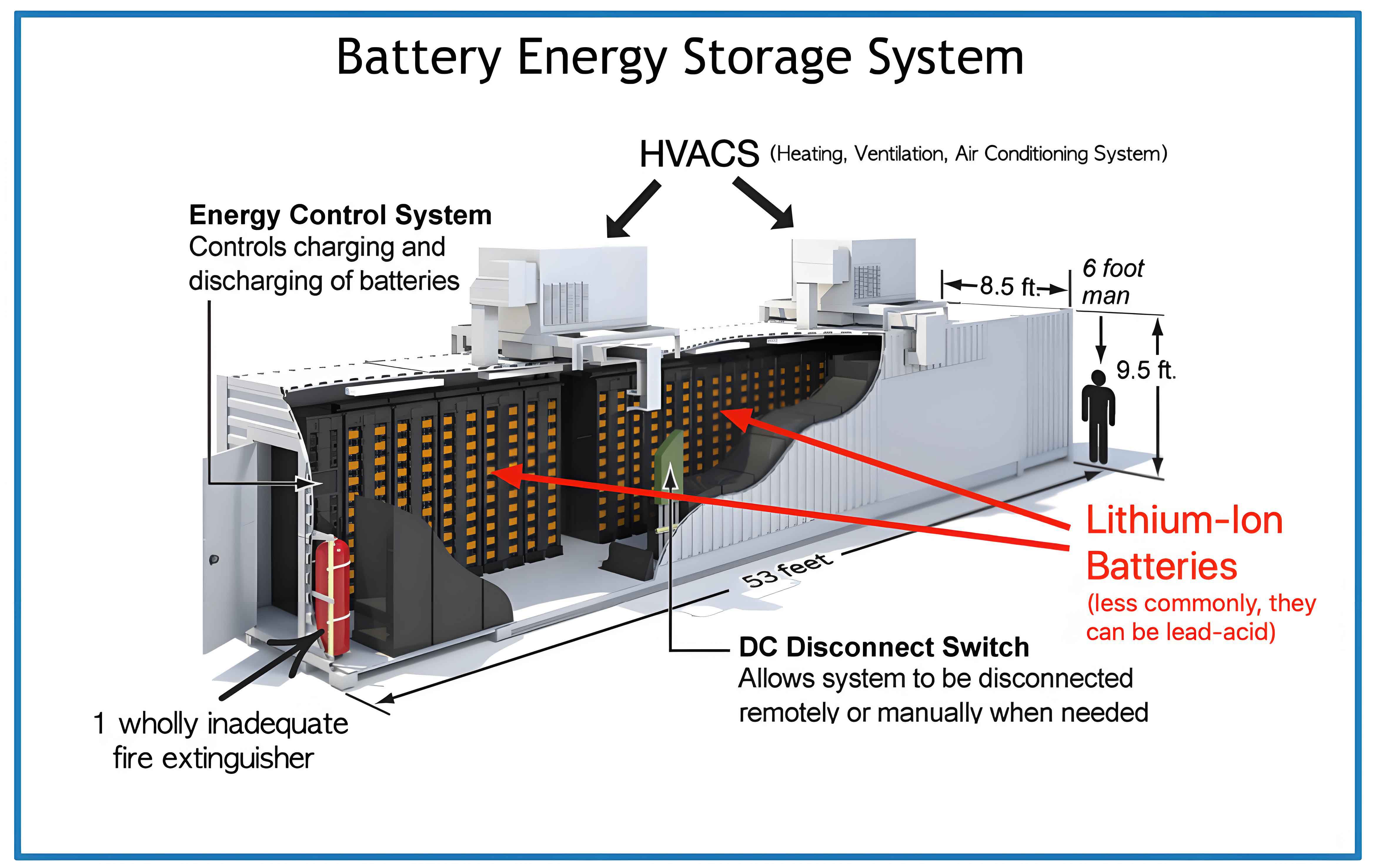
Lithium-ion batteries have mature technology, relatively low initial cost (1500~3000 yuan/kWh), and low maintenance costs, making them suitable for distributed short-term energy storage. Therefore, this study selects lithium batteries as the primary material for the energy storage system and conducts optimization configuration research on the Battery Energy Storage System (BESS).
2. Wind-Solar-Biogas-Storage Complementary Rural Distribution Network System Model
The “wind-solar-biogas-storage” complementary rural distribution network system constructed in this study consists of the following components: a distributed generation system comprising wind turbines, photovoltaic generators, and biomass gas turbine units; a chemical battery energy storage system with fast response and high-efficiency energy conversion capabilities along with a power conversion system; AC/DC loads and corresponding power electronic conversion equipment such as inverters.
The topology framework of the system is shown below.
In this system, the photovoltaic generator absorbs solar energy and outputs DC power, which is connected to the system’s AC grid through a DC/AC converter. The wind turbine converts wind energy into electrical energy, outputting AC power connected to the system’s AC grid through an AC/AC converter. The energy storage system is connected to the AC grid through a DC/AC converter. When the load demand is satisfied, the excess energy generated by photovoltaic and wind turbines is used to charge the energy storage system. When the system has a power deficit, the energy storage system discharges and transmits power to the load through the busbar.
2.1 Photovoltaic Output Power Mathematical Model
The photovoltaic power generation system converts solar radiation into electrical energy through the photovoltaic effect of solar cells. The output voltage U and output current I of the photovoltaic array satisfy the following mathematical model:
$$
I = I_{ph} – I_d – I_{sh}
$$
$$
I = I_{ph} – I_s \left[ \exp\left( \frac{q(U + IR_s)}{mk_B T} \right) – 1 \right] – \frac{U + IR_s}{R_{sh}}
$$
where $I_s$ is the leakage short-circuit current, $I_d$ is the reverse-direction current, $R_s$ and $R_{sh}$ are the series and parallel equivalent resistances respectively, $q$ is the electron charge, $k_B$ is the Boltzmann constant, and $T$ is the temperature.
According to the output mathematical model of photovoltaic cells:
$$
P_{PV}(t) = f_{PV} P_{PV} \frac{G(t)}{G_{STC}} \left[ 1 + \alpha_{PV}(T_{cell} – T_{cell-STC}) \right]
$$
where $P_{PV}(t)$ is the actual output power at time $t$, $P_{PV}$ is the rated output power, $f_{PV}$ is the derating factor, $G(t)$ is the solar radiation intensity at time $t$, $G_{STC}$ is the solar radiation intensity under standard test conditions, $\alpha_{PV}$ is the photovoltaic power temperature coefficient, $T_{cell}$ is the current operating temperature of the photovoltaic module, and $T_{cell-STC}$ is the temperature of the photovoltaic module under standard test conditions.
2.2 Wind Turbine Output Power Mathematical Model
The wind turbine generation system converts kinetic energy from wind into electrical energy. Based on actual wind speed conditions, the mathematical model of the wind power generation system is:
$$
P_{WT}(t) =
\begin{cases}
0 & 0 \leq v(t) \leq v_{ci} \\
P_{WT} \frac{v(t) – v_{ci}}{v_r – v_{ci}} & v_{ci} \leq v(t) \leq v_r \\
P_{WT} & v_r \leq v(t) \leq v_{co} \\
0 & v(t) \geq v_{co}
\end{cases}
$$
where $P_{WT}(t)$ is the actual output power of the wind turbine at time $t$, $P_{WT}$ is the rated output power, $v(t)$ is the wind speed at time $t$, $v_{ci}$ is the cut-in wind speed, $v_{co}$ is the cut-out wind speed, and $v_r$ is the rated wind speed.
2.3 Biogas Energy Output Power Mathematical Model
Biogas serves as a biomass energy carrier, converting agricultural waste into combustible gas with methane content of 55%~65% through anaerobic fermentation, driving a micro turbine to achieve efficient power generation. The power generation mathematical model is:
$$
P_{gas} = J \times \eta_{gas} \times F_{gas}
$$
where $P_{gas}$ is the output power of the micro turbine, $J$ is the theoretical combustion heat value of biogas, $\eta_{gas}$ is the power generation conversion efficiency of the micro turbine, and $F_{gas}$ is the flow rate of biogas.
The power mathematical model of the micro turbine is:
$$
P_{GAS}(t) = \left( \frac{P_{ho,t}}{\eta_h} + \frac{P_{co,t}}{\eta_c} \right) \cdot \eta_e \cdot (1 – \eta_{loss})
$$
where $P_{GAS}(t)$ is the output power of the micro turbine at time $t$, $\eta_h$ and $\eta_c$ are the thermal and cooling conversion coefficients of the micro turbine respectively, $\eta_e$ is the electrical power conversion coefficient, and $\eta_{loss}$ is the heat loss coefficient.
2.4 Energy Storage System Mathematical Model
The Thevenin equivalent circuit model of the battery is considered, where $E_m$ represents the open-circuit voltage, $R_s$ represents the internal resistance of the battery, and $R_p$ represents the polarization resistance. During the operation of the lithium battery, the state of charge is used to represent the remaining battery capacity:
$$
SOC(t) = \frac{E_{BESS}(t)}{E_{BESSmax}} \times 100\%
$$
where $E_{BESSmax}$ is the upper limit of battery energy storage capacity, and $SOC \in [0,1]$.
During battery charging:
$$
E_{BESS}(t) = E_{BESS}(t-1)(1-\delta) + P_{BESS,c}(t) \cdot \Delta t \cdot \eta_{BESS,s} \cdot \eta_{BESS,c} \cdot \eta_{PCS}
$$
During battery discharging:
$$
E_{BESS}(t) = E_{BESS}(t-1)(1-\delta) – P_{BESS,d}(t) \cdot \Delta t / (\eta_{BESS,c} \cdot \eta_{BESS,d} \cdot \eta_{DC-DC})
$$
The system incorporates a Power Conversion System (PCS), Energy Management System (EMS), and Supervisory Control And Data Acquisition (SCADA) system for collaborative control. The PCS controls the charge/discharge power to achieve energy interaction between the energy storage system and the grid.
3. Whale Optimization Algorithm and Its Improvement
3.1 Basic Whale Optimization Algorithm
The Whale Optimization Algorithm (WOA) is a meta-heuristic algorithm that simulates the hunting behavior of humpback whales. It has the advantages of simple structure and few parameters. WOA mainly includes three stages:
(1) Encircling prey:
$$
D = |C \cdot X_p(t) – X(t)|
$$
$$
X(t+1) = X_p(t) – A \cdot D
$$
where:
$$
A = 2a \cdot r_1 – a, \quad C = 2 \cdot r_2, \quad a = 2 – \frac{2t}{N_{max}}
$$
where $r_1, r_2 \in [0,1]$, and $N_{max}$ is the maximum number of iterations.
(2) Bubble-net attacking method:
$$
X(t+1) = D’ \cdot e^{bl} \cdot \cos(2\pi l) + X_p(t)
$$
where $b$ is a constant defining the shape of the logarithmic spiral, and $l \in [0,1]$.
(3) Search for prey:
$$
D = |C \cdot X_{rand}(t) – X(t)|
$$
$$
X(t+1) = X_{rand}(t) – A \cdot D
$$
3.2 Improved Whale Optimization Algorithm
To improve the diversity of the initial population, avoid falling into local optima, and further enhance algorithm performance, this study introduces a pooling mechanism to improve the search strategy of the whale algorithm, forming the Improved Whale Optimization Algorithm (IWOA).
(1) Pooling mechanism: The pooling mechanism acts as a crossover factor that fully mixes the optimal solution with the worst solution, increasing the diversity of solutions. For a matrix of size K, Pool = ($P_1, P_2, …, P_k$), each member $P_i = (P_{i,1}, P_{i,2}, …, P_{i,D})$ is generated after each iteration:
$$
P_i^t = B_i^t \times X_{best}^t + B_i^t \times X_{worst}^t
$$
where $B_i^t$ is a binary random vector.
(2) Migration search strategy: This strategy randomly separates some humpback whales to explore unvisited areas:
$$
X_i^{t+1} = X_{rnd}^t – X_{brnd}^t
$$
$$
X_{rnd}^t = rand \times (\delta_{max} – \delta_{min}) + \delta_{min}
$$
$$
X_{brnd}^t = rand \times (\delta_{best\_max} – \delta_{best\_min}) + \delta_{best\_min}
$$
(3) Elite selection search strategy: This strategy introduces a heavy-tailed Cauchy distribution to generate larger step sizes:
$$
X_i^{t+1} = X_i^t + A_i^t \times C_i^t \times (P_{rnd1}^t – P_{rnd2}^t)
$$
(4) Enriched encircling prey strategy:
$$
X_i^{t+1} = X_{best}^t – A_i^t \times D’^t
$$
$$
D’^t = |C_i^t \times X_{best}^t – P_{rnd3}^t|
$$
(5) Vertical crossover strategy: The vertical crossover operation is performed on two different dimensions of the global optimal solution. The crossover process for the $d_1$-th and $d_2$-th dimensions of $X_i^T$ is:
$$
M_{X_{i,d}}^T = m \times X_{i,d_1}^T + (1-m) \times X_{i,d_2}^T
$$
where $M_{X_{i,d}}^T$ is the offspring individual generated by the vertical crossover, and $m \in [0,1]$.
3.3 Performance Testing of IWOA
To verify the optimization performance of the IWOA algorithm, this section selects 9 benchmark functions, where $F_1$, $F_2$, $F_3$ are unimodal functions, $F_4$, $F_5$, $F_6$ are multimodal functions, and $F_7$, $F_8$, $F_9$ are fixed-dimension multimodal functions. The algorithm parameters are set as follows: population size = 30, maximum iterations = 500.
| Algorithm | Parameter | Value |
|---|---|---|
| PSO | $V_{max}$, $c_1$, $c_2$ | 6, 2 |
| GWO and IGWO | $a$ | [0, 2] |
| SOA | $f_c$, $A$ | 2, [0, 2] |
| WOA and IWOA | $W_f$ | [0.05, 0.1] |
| Function | Dimension | Search Range | Minimum |
|---|---|---|---|
| $F_1(x) = \sum_{i=1}^{n} x_i^2$ | 30 | [-100, 100] | 0 |
| $F_2(x) = \sum_{i=1}^{n} |x_i| + \prod_{i=1}^{n} |x_i|$ | 30 | [-10, 10] | 0 |
| $F_3(x) = \sum_{i=1}^{n-1} [100(x_{i+1} – x_i^2)^2 + (x_i – 1)^2]$ | 30 | [-30, 30] | 0 |
| $F_4(x) = \sum_{i=1}^{n} [x_i^2 – 10\cos(2\pi x_i) + 10]$ | 30 | [-5.12, 5.12] | 0 |
| $F_5(x) = -20\exp(-0.2\sqrt{\frac{1}{n}\sum_{i=1}^{n} x_i^2}) – \exp(\frac{1}{n}\sum_{i=1}^{n} \cos(2\pi x_i)) + 20 + e$ | 30 | [-32, 32] | 0 |
| $F_6(x) = \frac{\pi}{n}\{10\sin(\pi y_1) + \sum_{i=1}^{n-1}(y_i – 1)^2[1 + 10\sin^2(\pi y_{i+1})] + (y_n – 1)^2\} + \sum_{i=1}^{n} u(x_i, 10, 100, 4)$ | 30 | [-50, 50] | 0 |
| $F_7(x) = \sum_{i=1}^{11} [a_i – \frac{x_1(b_i^2 + b_i x_2)}{b_i^2 + b_i x_3 + x_4}]^2$ | 4 | [-5, 5] | 0.1484 |
| $F_8(x) = -\sum_{i=1}^{4} c_i \exp[-\sum_{j=1}^{3} a_{ij}(x_j – p_{ij})^2]$ | 3 | [1, 3] | -3 |
| $F_9(x) = -\sum_{i=1}^{5} [(X – a_i)(X – a_i)^T + c_i]^{-1}$ | 4 | [0, 10] | -1 |
The test results are presented in the following table:
| Function | Metric | PSO | GWO | IGWO | SOA | WOA | IWOA |
|---|---|---|---|---|---|---|---|
| $F_1$ | Best | 7.6611 | 0.0643 | 57.8057 | 1.8958e-38 | 4.0561e-15 | 0 |
| Aver | 78.6611 | 0.0794 | 9.7070 | 2.9552e-40 | 4.7041e-16 | 0 | |
| STD | 65.2674 | 0.0563 | 23.6878 | 8.8713e-39 | 3.6783e-15 | 0 | |
| $F_2$ | Best | 1.3621e-06 | 0.0040 | 6.9573 | 7.9077e-40 | -2.8197e-18 | 0 |
| Aver | 2.6417e-06 | 0.0037 | 0.4171 | 8.6816e-42 | -6.8979e-19 | 0 | |
| STD | 3.7411e-07 | 0.0002 | 2.5532 | 2.5233e-40 | 1.8793e-18 | 0 | |
| $F_7$ | Best | 0.2145 | 0.3485 | 0.2775 | 0.1231 | 0.1580 | 0.0135 |
| Aver | 0.1942 | 0.3357 | 2.1325 | 0.1606 | 0.2004 | 0.1613 | |
| STD | 1.5792 | 1.5568 | 1.5678 | 0.0364 | 0.0545 | 0.0365 | |
| $F_8$ | Best | -3.3475 | -3.3216 | 0.0103 | 0.1468 | 0.0381 | -3.4715 |
| Aver | -3.2031 | -3.2031 | 0.3768 | 0.3449 | 0.4773 | -3.2187 | |
| STD | 0.1478 | 0.1268 | 0.2624 | 0.1901 | 0.3563 | 0.00452 | |
| $F_9$ | Best | -5.0876 | -5.0876 | 2.6529 | 3.9995 | -5.0876 | -5.0876 |
| Aver | -4.0165 | -4.2753 | 3.7935 | 4.0001 | 3.9999 | -5.0876 | |
| STD | 2.0114 | 1.4526 | 1.2072 | 1.4442 | 0.0033 | 0.0001115 |
The Wilcoxon rank-sum test results are as follows:
| Function | PSO | GWO | IGWO | SOA | WOA |
|---|---|---|---|---|---|
| $F_1$ | 7.0056e-08 | 7.0056e-08 | 7.0056e-08 | 7.0056e-08 | 7.0056e-08 |
| $F_2$ | 7.0056e-08 | 7.0056e-08 | 7.0056e-08 | 7.0056e-08 | 7.0056e-08 |
| $F_3$ | 7.0056e-08 | 7.0056e-08 | 7.0056e-08 | 7.0056e-08 | NaN |
| $F_4$ | 7.0056e-08 | 1.0379e-06 | 0.0057266 | 7.0056e-08 | NaN |
| $F_5$ | 7.0056e-08 | 5.6751e-07 | 8.3578e-09 | 7.0045e-08 | NaN |
| $F_6$ | 7.0056e-08 | 7.0056e-08 | 7.0056e-08 | 7.0056e-08 | NaN |
| $F_7$ | 5.4512e-07 | 0.91423 | 3.142e-06 | 5.6418e-07 | 3.3477e-06 |
| $F_8$ | 6.3041e-04 | 0.10641 | 0.54133 | 5.6418e-07 | 7.4751e-05 |
| $F_9$ | 2.6741e-04 | 6.545e-07 | 0.0080412 | 5.6418e-07 | 6.7861e-07 |
The p-values for all five comparison algorithms across the 9 benchmark functions are significantly less than 0.05, proving that IWOA has statistically significant differences from the other 5 algorithms, demonstrating that its optimization performance is statistically significant.
4. Multi-Objective Optimal Configuration Modeling and Solution of Energy Storage Systems in Rural Distribution Networks
A bilevel programming model has a two-layer hierarchical structure. The inner and outer layers set corresponding objective functions and constraints according to optimization needs. The long-time-scale energy storage system planning problem is placed in the outer layer model, while the short-time-scale operation problem is handled in the inner layer model.
Outer layer decision model:
$$
\min_x F_h(x, y) \quad h=1,2,3
$$
$$
\text{s.t.} \quad G(x, y) \leq 0
$$
Inner layer decision model:
$$
\min_y f(x, y)
$$
$$
\text{s.t.} \quad g(x, y) \leq 0
$$
4.1 Outer Layer Optimization Objective Function Model
The outer layer takes the annual investment and operation maintenance cost, voltage stability, and load fluctuation optimization as the main objectives, constructing a multi-objective model based on Pareto optimization.
(1) Annual investment operation and maintenance cost:
$$
F_1 = C_{tcc} + C_{om} + C_{p-s} – C_{sub} – C_{envi}
$$
where $C_{tcc}$, $C_{om}$ and $C_{p-s}$ are the annual investment cost, operation and maintenance cost, and charge/discharge cost of the energy storage system respectively; $C_{sub}$ is the government subsidy for generated electricity; $C_{envi}$ is the environmental benefit.
$$
C_{tss} = \sum_{j=1}^{N} [\mu \cdot (C_{inv} + \mu_{BESS,E} \cdot E_{BESS} + \mu_{BESS,P} \cdot P_{BESS})]
$$
where $N$ is the number of energy storage systems, $C_{inv}$ is the investment cost of a single energy storage system, $\mu_{BESS,E}$ and $\mu_{BESS,P}$ represent the unit capacity cost and unit power cost of the energy storage system respectively, and $\mu$ is the annual capital recovery rate:
$$
\mu = \frac{\rho(1+\rho)^y}{(1+\rho)^y – 1}
$$
where $y$ is the investment period and $\rho$ is the discount rate.
$$
C_{om} = \sum_{j=1}^{N} [\rho_{om} \cdot (\mu_{BESS,E} \cdot E_{BESS} + \mu_{BESS,P} \cdot P_{BESS})]
$$
$$
C_{p-s} = \sum_{j=1}^{N} \sum_{t=1}^{T} [\rho_{sell}(t) \cdot P_{BESS,c}(t) – \rho_{out}(t) \cdot P_{BESS,d}(t)]
$$
$$
C_{sub} = \lambda \cdot \sum_{j=1}^{N} \sum_{t=1}^{T} P_{BESS,d}(t)
$$
$$
C_{envi} = \sum_{t=1}^{T} \Delta P_{grid}(t) \cdot Y \cdot D_{grid}
$$
(2) Annual total voltage fluctuation: The grid vulnerability index is introduced to reduce the limitations of directly introducing node voltages. The vulnerability of each node is quantified with the addition of weight indicators:
$$
F_2 = \sum_{t=1}^{T} [\lambda_1 BV(t) + \lambda_2 J(t)]
$$
where $BV(t)$ is the average grid vulnerability, $J(t)$ is the equilibrium degree of vulnerability distribution at each node, and $\lambda_1 = \lambda_2 = 0.5$.
$$
BV(t) = \frac{1}{N} \sum_{i=1}^{N} V(t,i)
$$
$$
J(t) = -\sum_{i=1}^{N} \frac{p_{t,i}}{\log_2} \log_2 \left( \frac{p_{t,i}}{\log_2 N} \right)
$$
The normalized vulnerability value of node $i$ at time $t$ is:
$$
V(t,i) = \frac{v(t,i) – v(t,i_{min})}{v(t,i_{max}) – v(t,i_{min})}
$$
$$
v(t,i) = \frac{1 – U(t,i)}{U(t,0)} \cdot A
$$
where $U(t,i)$ and $U(t,0)$ are the voltage of node $i$ and the rated voltage respectively, and $A=0.007$.
(3) Annual total load fluctuation:
$$
F_3 = \frac{\sum_{t=1}^{T} (P_{load}(t) – P_{WT}(t) – P_{PV}(t) – P_{GAS}(t) – \overline{P_L})^2}{T}
$$
4.2 Outer Layer Optimization Constraints
(1) Power balance constraint:
$$
P_{load}(t) = P_{WT}(t) + P_{PV}(t) + P_{GAS}(t) + P_{BESS,c/d}(t) + P_{grid}(t)
$$
$$
Q_{load}(t) = Q_{WT}(t) + Q_{PV}(t) + Q_{GAS}(t) + Q_{BESS,c/d}(t) + Q_{grid}(t)
$$
(2) Voltage constraint:
$$
V_i^{min} \leq V_i \leq V_i^{max}
$$
(3) Tie-line power constraint:
$$
P_{grid}^{min}(t) \leq P_{grid}(t) \leq P_{grid}^{max}(t)
$$
$$
Q_{grid}^{min}(t) \leq Q_{grid}(t) \leq Q_{grid}^{max}(t)
$$
(4) Energy storage system capacity and power constraints:
$$
E_{BESS}^{min}(t) \leq E_{BESS,n}(t) \leq E_{BESS}^{max}(t)
$$
$$
P_{BESS}^{min}(t) \leq P_{BESS,n}(t) \leq P_{BESS}^{max}(t)
$$
4.3 Inner Layer Optimization Objective Function Model
The inner layer optimizes the loss cost of the energy storage system, considering only the depth of charge/discharge and cycle times:
$$
f = \sum_{j=1}^{N} \sum_{t=1}^{T} C_{BESS}^{life} \cdot \eta_{BESS,d} \cdot P_{BESS,d}(t) + C_{BESS}^{life} \cdot \eta_{BESS,c} \cdot P_{BESS,c}(t)
$$
The loss cost of a single battery is:
$$
C_{BESS}^{life} = C_E \cdot |SOC_{aux}(t) – SOC(t-1)|
$$
where $C_E$ is the single-cycle degradation cost of the energy storage system:
$$
C_E = \frac{C_{inv}}{N_{cycle}}
$$
The relationship between the depth of discharge (DOD) and cycle life is:
$$
N_{cycle} = 1788 \cdot DOD^{0.6486} \cdot \exp[5.021(1 – DOD)]
$$
4.4 Inner Layer Optimization Constraints
(1) Charge/discharge constraints:
$$
P_{BESS}^{min} \leq P_{BESS,n}(t) \leq P_{BESS}^{max}
$$
$$
E_{BESS}^{min} \leq E_{BESS,n}(t) \leq E_{BESS}^{max}
$$
(2) SOC constraint:
$$
SOC^{min} \leq SOC(t) \leq SOC^{max}
$$
4.5 Multi-Objective Improved Whale Optimization Algorithm
Based on the Pareto dominance principle and the IWOA algorithm, a Multi-Objective Improved Whale Optimization Algorithm (MOIWOA) is designed. The key lies in effectively handling multiple objective function models and managing and screening the Pareto frontier solution set.
For the diversity of the Pareto solution set, the following formula is used to determine whether the distribution of non-dominated solutions is compact:
$$
\zeta =
\begin{cases}
\frac{F(x_i) – F(x_j)}{F^{max} – F^{min}} < N_r \\
\zeta = \frac{F(x_i) – F(x_j)}{F^{max} – F^{min}}
\end{cases}
$$
4.6 Improved Ideal Point Decision Method
To address the problem of different dimensions among multiple objective functions in the Pareto solution set, normalization is performed:
$$
u_i^k = \frac{f_i(x_k) – f_i^{min}}{f_i^{max} – f_i^{min}}
$$
The ideal target point is $O(0,0,0)$. To reduce the interference of human subjective preferences in the decision-making process, an Improved Ideal-Point Based Decision (IIPBD) method is proposed to select the optimal compromise solution. The mathematical model is:
$$
X_k = \sum_{i=1}^{m} \left| u_i^k – O \right|^2
$$
By comparing the minimum value of the squared Euclidean distance of each Pareto non-dominated solution across each objective, the optimal compromise solution is determined.
5. Simulation and Analysis of Energy Storage System Optimal Configuration in Rural Distribution Networks
5.1 High-Proportion New Energy Scenario Generation
The Savitzky-Golay filter is used for data preprocessing. This method is based on a local polynomial regression framework, establishing a high-order polynomial approximation model within a sliding window. The data points $x_i$ within the window are constructed through an $n$-order polynomial:
$$
f(i) = \sum_{j=0}^{n} a_j i^j = a_0 + a_1 i + a_2 i^2 + \cdots + a_n i^n
$$
The residual sum of squares is:
$$
E = \sum_{j=-m}^{m} (f(i) – x_i)^2 = \sum_{j=-m}^{m} \left( \sum_{j=0}^{n} a_j i^j – x_i \right)^2
$$
The kernel density estimation is used to construct the output probability distribution model. The Gaussian kernel function is:
$$
K_h(x, \theta) = \frac{1}{\sqrt{2\pi}\theta} e^{-\frac{x^2}{2\theta^2}}
$$
The bandwidth parameter is determined by:
$$
\theta \approx 1.06 \delta n^{-0.2}
$$
The probability density function is:
$$
f(x) = \frac{1}{n} \sum_{i=1}^{n} K_h(x – X_i) = \frac{1}{n\theta} \sum_{i=1}^{n} \frac{x – X_i}{\theta}
$$
Using Latin Hypercube Sampling and the improved K-Means clustering algorithm, typical operating scenario sets are generated. The annual output curves are shown in the following figure.
The wind, solar, and load output curves under 5 typical scenarios are obtained. The probabilities of each scenario are:
| Typical Scenario | Scenario 1 | Scenario 2 | Scenario 3 | Scenario 4 | Scenario 5 |
|---|---|---|---|---|---|
| $P_{WIND}$ | 0.170 | 0.208 | 0.272 | 0.204 | 0.146 |
| $P_{PV}$ | 0.254 | 0.186 | 0.206 | 0.207 | 0.147 |
| $P_{LOAD}$ | 0.218 | 0.190 | 0.162 | 0.184 | 0.246 |
5.2 Simulation Parameters and Model
A rural distribution network with a rated voltage level of 10kV is used as the case study. The node voltage per-unit value range is [0.93pu, 1.07pu]. The total load is (3.14+j1.7)MVA. Wind turbines with capacity of 200kW are connected at nodes 14 and 19, while photovoltaic generators with capacity of 200kW are connected at nodes 3 and 12. A biogas power generation plant is located at node 17.
Two energy storage systems are configured at different nodes from node 2 to node 28. The parameters of the energy storage system are:
| Parameter | Symbol | Value |
|---|---|---|
| Fixed construction cost (10k yuan/unit) | $C_{ap}$ | 100 |
| Unit power cost (10k yuan/MW) | $\mu_{BESS,E}$ | 95 |
| Unit capacity cost (10k yuan/MWh) | $\mu_{BESS,P}$ | 98; 180; 314; 580 |
| Electricity generation subsidy coefficient (10k yuan/MW) | $\lambda$ | 0.01 |
| Operation and maintenance cost coefficient | $\rho_{om}$ | 0.05 |
| Discount rate coefficient | $\rho$ | 0.0633 |
| Charging efficiency | $\eta_{BESS,c}$ | 0.95 |
| Discharging efficiency | $\eta_{BESS,d}$ | 0.95 |
| Self-discharge rate | $\delta$ | 0.01 |
| SOC minimum | $SOC_{min}$ | 0.2 |
| SOC maximum | $SOC_{max}$ | 0.9 |
The time-of-use electricity price is as follows:
| Time Period | Selling Price (thousand yuan/MWh) | Purchasing Price (thousand yuan/MWh) |
|---|---|---|
| 00:00-08:00 | 0.17 | 0.13 |
| 08:00-11:00 | 0.49 | 0.38 |
| 11:00-16:00 | 0.83 | 0.65 |
| 16:00-19:00 | 0.49 | 0.38 |
| 19:00-22:00 | 0.83 | 0.65 |
| 22:00-24:00 | 0.49 | 0.38 |
5.3 Algorithm Performance Evaluation
To evaluate the performance of the proposed MOIWOA-IWOA in the multi-objective optimization problem of the energy storage system, the simulation compares three traditional algorithms: MOPSO-PSO, NSGAII-GA, and MOWOA-WOA. All algorithms have a maximum iteration of 100, a population size of 100, and an external archive size of 20.
The numerical results of the Pareto non-dominated solution sets obtained by the four algorithms are:
| Algorithm | Objective Function | $F_1$/(10^6 yuan) | $F_2$/(p.u.) | $F_3$/(MW) |
|---|---|---|---|---|
| MOPSO-PSO | Optimal value | 2.442 | 0.241 | 330.414 |
| Worst value | 5.247 | 0.615 | 499.143 | |
| Average value | 3.987 | 0.473 | 420.471 | |
| NSGAII-GA | Optimal value | 2.135 | 0.227 | 317.521 |
| Worst value | 4.912 | 0.483 | 457.514 | |
| Average value | 3.912 | 0.427 | 391.154 | |
| MOWOA-WOA | Optimal value | 2.014 | 0.195 | 299.154 |
| Worst value | 4.871 | 0.474 | 422.213 | |
| Average value | 3.821 | 0.411 | 382.145 | |
| MOIWOA-IWOA | Optimal value | 1.994 | 0.214 | 264.133 |
| Worst value | 4.775 | 0.408 | 411.715 | |
| Average value | 3.785 | 0.375 | 318.640 |
To further verify the quality of the Pareto non-dominated solution sets obtained by MOIWOA-IWOA, five indicators are used for quantitative evaluation: Generational Distance (GD), Inverted Generational Distance (IGD), Diversity Metric (DM), Spacing (SP), and Hyper Volume (HV).
| Algorithm | GD (×10⁴) | IGD (×10⁴) | DM | SP (×10⁴) | HV |
|---|---|---|---|---|---|
| MOPSO-PSO | 2.238 | 2.854 | 0.821 | 5.125 | 0.065 |
| NSGAII-GA | 2.451 | 2.415 | 0.811 | 2.214 | 0.081 |
| MOWOA-WOA | 2.115 | 1.213 | 0.795 | 2.416 | 0.078 |
| MOIWOA-IWOA | 0.752 | 1.242 | 0.841 | 2.115 | 0.114 |
The GD, IGD, and SP values of MOIWOA-IWOA are relatively small, indicating that MOIWOA-IWOA has good convergence and a more uniform distribution of Pareto solutions. The DM and HV values are the largest, indicating that the Pareto solution set is richer and more diverse than the other three algorithms.
5.4 Energy Storage System Optimal Configuration Analysis
Based on the MOIWOA-IWOA solution and the IIPBD method, the optimal configuration scheme of the energy storage system is obtained:
| Inner Layer Optimization Result f/(10⁴ yuan) | Outer Layer Optimization Result | ||||||
|---|---|---|---|---|---|---|---|
| Installation Nodes | Power/(MW) | Capacity/(MWh) | Inner f/(10⁴ yuan) | $F_1$/(10⁶ yuan) | $F_2$/(p.u.) | $F_3$/(MW) | |
| (24, 6) | (0.327, 0.284) | (1.426, 1.353) | 0.421 | 3.538 | 0.357 | 304.874 | |
The spatial hierarchical layout strategy deploys the first energy storage system at the load density peak area, undertaking the core functions of load shifting and voltage support. The second energy storage system is deployed adjacent to the main grid interaction node to achieve cross-area power balance and market revenue targets, participating in peak-valley arbitrage and frequency regulation auxiliary services.
5.5 Operation Status Analysis of the Energy Storage System
The analysis of the operation status of the two energy storage systems shows: (1) both energy storage systems maintain high utilization rates, operating almost throughout the day, ensuring that the SOC values of each system remain at 0.5 at both the start and end times; (2) the charge/discharge depths of both systems are reasonable, with SOC values fluctuating within the range of [0.2, 0.9], ensuring the lithium battery achieves the expected service life; (3) the SOC of the two storage units exhibits dynamic equilibrium characteristics, with the daytime SOC fluctuation ranges of the first and second energy storage systems being [0.32, 0.67] and [0.28, 0.64] respectively.
Under the dynamic time-of-use electricity price mechanism, the first energy storage system focuses on load node pressure mitigation, performing stepped charging during valley periods (00:00-08:00), maintaining standby during flat periods (08:00-11:00), and releasing energy during peak periods. The second energy storage system is deployed at the main grid interaction node, executing peak-valley arbitrage, returning power to the main grid during peak price periods (11:00-16:00 and 19:00-22:00, 0.83 thousand yuan/kWh).
5.6 Technical Benefit Analysis of the Energy Storage System
Two scenarios are set for comparison: with and without the energy storage system. The results are as follows:
The average voltage levels of all nodes in the rural distribution network system before and after configuring the energy storage system are compared. The equivalent load levels of the system over 24 hours before and after configuration are also analyzed. The comparison yields the following conclusions:
(1) Through reasonable configuration of the energy storage system, the system voltage level has improved, and the overall voltage quality has been significantly optimized. The local voltage of the rural distribution network has been improved, especially the voltage at the end of the line. For the annual total voltage deviation, before the energy storage system was connected, it was 4812.5p.u., and after the energy storage system was connected, it decreased to 4042.3p.u., a reduction of 16.01%.
(2) Reasonable configuration of the energy storage system reduced the equivalent load level of the system, lowering the load fluctuation caused by the large load difference and high-proportion new energy output. The annual load standard deviation after connecting the energy storage system was reduced from 0.471MW to 0.455MW, a decrease of 3.40%.
The above analysis verifies that reasonable configuration of the energy storage system can suppress voltage fluctuations, improve system voltage levels, and simultaneously suppress system load fluctuations, thereby enhancing system stability.
5.7 Economic Benefit Analysis of the Energy Storage System
The economic benefits brought by the energy storage system configuration are evaluated. The main sources are the low-storage high-discharge arbitrage, government subsidies, and additional benefits such as carbon emission reduction benefits.
| Economic Benefit | Annual Investment Cost of BESS/(10k yuan) | Annual O&M Cost of BESS/(10k yuan) | Arbitrage Revenue/(10k yuan) | Government Subsidy/(10k yuan) |
|---|---|---|---|---|
| After BESS integration | 160.79 | 85.6 | 35.57 | 12.23 |
With the optimized configuration scheme, the annual carbon emission cost before and after configuring the energy storage system decreased from 5.83 to 5.21 ten thousand yuan, a reduction of 10.6%. The energy storage system can generate a total profit of 47.8 ten thousand yuan annually through low-storage high-discharge arbitrage and government subsidies. Over the 15-year investment period, the energy storage system can generate a cumulative profit of 717 ten thousand yuan.
6. Conclusion and Outlook
This study focuses on the optimal configuration of energy storage systems in rural distribution networks with high-penetration renewable energy integration. The main contributions and conclusions are as follows:
(1) A “wind-solar-biogas-storage” complementary rural distribution network system model was constructed, and the technical and economic benefits of integrating the energy storage system were theoretically analyzed. Lithium battery energy storage technology was selected as the storage medium based on comprehensive technical and economic comparisons.
(2) An Improved Whale Optimization Algorithm (IWOA) was proposed by introducing a pooling mechanism to increase population diversity and a heavy-tailed Cauchy distribution to avoid falling into local optima. Benchmark tests on 9 functions with comparisons against 5 classical algorithms and 3 hybrid algorithms verified the superiority of IWOA in global search capability, solution quality, optimization accuracy, and convergence speed.
(3) A bilevel multi-objective optimization configuration model was established, minimizing annual investment operation and maintenance costs, grid vulnerability, and annual load fluctuation indicators in the outer layer, while quantifying the service life of the energy storage system in the inner layer. A Pareto-based multi-objective improved whale algorithm (MOIWOA-IWOA) was designed to solve the model, with an improved ideal point decision method for objective selection of the compromise solution.
(4) Simulation results on a rural distribution network case demonstrate that the proposed MOIWOA-IWOA achieves superior Pareto solution set quality with better distribution uniformity compared to three benchmark algorithms. The optimized energy storage system configuration reduced the annual total voltage deviation by 16.01% and improved the load fluctuation rate by 3.40%, while bringing considerable economic benefits through arbitrage and subsidies.
Future research directions may include: considering more complex energy storage degradation mechanisms such as temperature effects; developing more efficient algorithms to address the computational burden of bilevel multi-objective optimization; and incorporating demand-side response and electric vehicle integration into the rural distribution network optimization framework.