
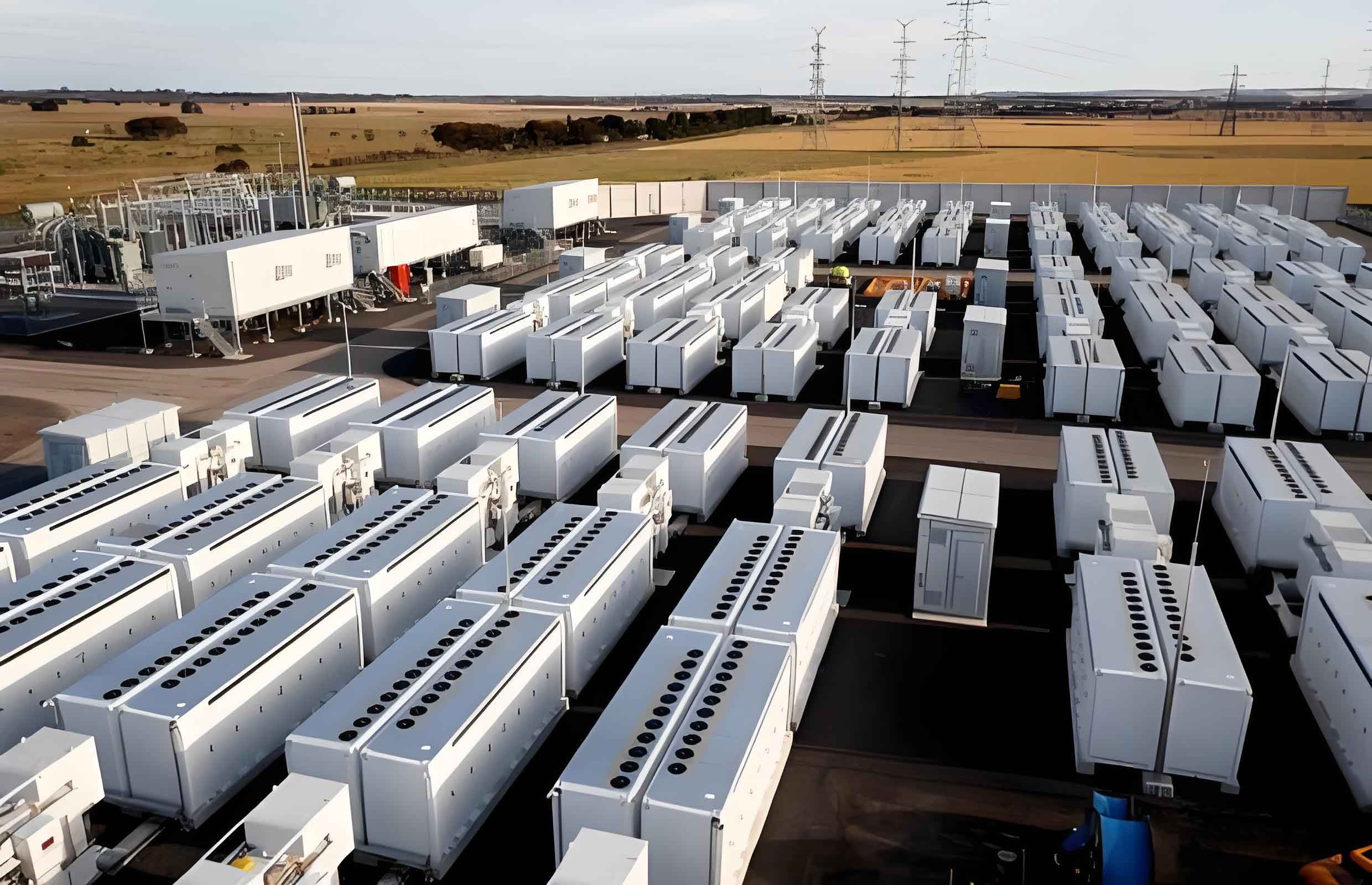
As an emerging technology in the field of energy storage, the all-vanadium redox flow battery has attracted widespread attention due to its excellent safety, long cycle life, flexible design, and environmental friendliness. In the context of global carbon neutrality goals and the rapid expansion of renewable energy integration, the energy storage battery systems based on vanadium redox flow technology have demonstrated tremendous potential for large-scale long-duration energy storage applications. However, during the charge-discharge cycle, the battery continuously generates heat, and once the operating temperature exceeds the safe range, the electrolyte tends to precipitate. Such precipitation can lead to multiple failures including reduced battery efficiency, blocked flow channels, and even catastrophic battery failure. Therefore, real-time temperature monitoring of the energy storage battery is of paramount importance. This research focuses on the temperature sensing problem of vanadium redox flow batteries, conducting systematic investigations from three aspects: multi-physics finite element numerical simulation, distributed optical fiber temperature monitoring, and internal spatial temperature prediction of the battery.
1. Multi-Physics Coupling Modeling of the Vanadium Redox Flow Battery
To accurately capture the temperature distribution characteristics of the energy storage battery, I established a three-dimensional multi-physics coupling finite element model of a single cell from a 10 kW vanadium redox flow battery stack. The model incorporates electrochemical reactions, fluid flow, and heat transfer phenomena simultaneously. Since the length-width dimensions of a single cell are an order of magnitude larger than the thickness direction, I scaled down the cell dimensions by a factor of 10 in the length and width directions while maintaining the original thickness. This simplification allows for efficient computation while preserving the essential thermal behavior of the energy storage battery system.
1.1 Model Geometry and Material Parameters
The structural dimensions of the modeled single cell are shown in Table 1. The model consists of seven parts arranged from the inside outward: the negative graphite electrode, the negative flow channel, the negative electrode frame, the proton exchange membrane, the positive electrode, the positive flow channel, and the positive electrode frame. The electrolyte enters from the bottom of the electrode through the flow channel and exits from the top.
| Component | Length (mm) | Width (mm) | Thickness (mm) |
|---|---|---|---|
| Electrode | 40 | 40 | 3 |
| Flow channel | 4 | 2 | 3 |
| Proton exchange membrane | 40 | 40 | 0.125 |
| Electrode frame | 48 | 48 | 3 |
The material properties used in the simulation are summarized in Table 2. The electrodes are made of porous graphite felt with a high porosity of 0.929, which allows for sufficient electrolyte flow and provides active reaction sites. The proton exchange membrane is a Nafion 212 membrane, and the electrode frame is made of polyvinyl chloride.
| Parameter | Value | Unit |
|---|---|---|
| Electrode density | 100 | kg/m³ |
| Electrode thermal conductivity | 0.15 | W/m·K |
| Electrode specific heat capacity | 710 | J/kg·K |
| Electrode electrical conductivity | 6000 | S/m |
| Electrode specific surface area | 1.62×10⁴ | m²/m³ |
| Electrode porosity | 0.929 | – |
| Electrolyte density | 1354 | kg/m³ |
| Electrolyte thermal conductivity | 0.67 | W/m·K |
| Electrolyte specific heat capacity | 4187 | J/kg·K |
| Membrane thermal conductivity | 0.67 | W/m·K |
| Membrane density | 1967 | kg/m³ |
| Membrane specific heat capacity | 3000 | J/kg·K |
| Dynamic viscosity of electrolyte | 4.298×10⁻³ | Pa·s |
1.2 Governing Equations
The multi-physics model of the energy storage battery is governed by a set of partial differential equations describing the conservation of mass, momentum, charge, species, and energy. For the electrolyte flow in the flow channels, I applied the incompressible Navier-Stokes equations:
$$\nabla \cdot \mathbf{v} = 0 \tag{1}$$
$$\rho(\mathbf{v} \cdot \nabla)\mathbf{v} = -\nabla P + \mu \nabla^2 \mathbf{v} \tag{2}$$
where ρ is the electrolyte density, P is the pressure, v is the velocity vector, and μ is the dynamic viscosity.
For the porous electrode regions, I employed the Brinkman equation, which provides better numerical stability:
$$\frac{\mu}{K}\mathbf{v} = -\nabla P + \mu^* \nabla^2 \mathbf{v} \tag{3}$$
where K is the permeability of the porous medium, described by the Carmen-Kozeny equation:
$$K = \frac{d_f^2 \varepsilon^3}{16 k_{CK} (1-\varepsilon)^2} \tag{4}$$
where ε is the electrode porosity, df is the average fiber diameter, and kCK is the Carmen-Kozeny constant.
For charge conservation, I applied Ohm’s law in both the solid electrode phase and the electrolyte phase:
$$\nabla \cdot i_s + \nabla \cdot i_l = 0 \tag{5}$$
$$i_s = -\sigma_s^{eff} \nabla \phi_s \tag{6}$$
$$i_l = -\kappa_l^{eff} \nabla \phi_l \tag{7}$$
where σseff is the effective electronic conductivity and κleff is the effective ionic conductivity. The effective conductivities are corrected using Bruggemann’s correlation:
$$\sigma_s^{eff} = \sigma_s (1-\varepsilon)^{3/2} \tag{8}$$
For species conservation, the mass transport in the electrolyte is described by:
$$\nabla \cdot (-D_i^{eff} \nabla c_i + \mathbf{v} c_i) = S_i \tag{9}$$
where ci is the concentration of species i (V²⁺, V³⁺, VO²⁺, VO₂⁺), Dieff is the effective diffusion coefficient, and Si is the source term associated with the electrochemical reactions.
The electrochemical reactions are described by the Butler-Volmer equation. For the positive electrode:
$$j_1 = F k_1 (c_5)^{\alpha_{Pa}} (c_4)^{\alpha_{Pc}} \left[ \exp\left(\frac{\alpha_{Pa} F \eta_1}{RT}\right) – \exp\left(-\frac{\alpha_{Pc} F \eta_1}{RT}\right) \right] \tag{10}$$
For the negative electrode:
$$j_2 = F k_2 (c_3)^{\alpha_{Na}} (c_2)^{\alpha_{Nc}} \left[ \exp\left(\frac{\alpha_{Na} F \eta_2}{RT}\right) – \exp\left(-\frac{\alpha_{Nc} F \eta_2}{RT}\right) \right] \tag{11}$$
where η represents the overpotential, F is Faraday’s constant, R is the universal gas constant, and T is the temperature. The overpotentials are defined as:
$$\eta_1 = \phi_s – \phi_l – E_1 \tag{12}$$
$$\eta_2 = \phi_s – \phi_l – E_2 \tag{13}$$
The Nernst equation is used to calculate the open-circuit potentials:
$$E_1 = E_0^+ + \frac{RT}{F} \ln\left(\frac{c_5}{c_4}\right) \tag{14}$$
$$E_2 = E_0^- + \frac{RT}{F} \ln\left(\frac{c_3}{c_2}\right) \tag{15}$$
The energy conservation equation accounts for three heat generation mechanisms: reversible reaction heat (qR), activation heat (qA), and ohmic heat (qO):
$$\rho C_p \mathbf{v} \cdot \nabla T = \nabla \cdot (\lambda \nabla T) + q_R + q_A + q_O \tag{16}$$
The source terms for the energy equation are summarized in Table 3.
| Source term | Positive electrode | Negative electrode | Membrane |
|---|---|---|---|
| qR | a j₁ (−ΔS₁ T / F) | a j₂ (−ΔS₂ T / F) | 0 |
| qO | σseff|∇φs|² + κleff|∇φl|² | σseff|∇φs|² + κleff|∇φl|² | κmeff|∇φm|² |
| qA | a j₁ η₁ | a j₂ η₂ | 0 |
1.3 Boundary Conditions and Mesh Generation
For the momentum conservation, I applied a velocity boundary condition at the flow channel inlet and a pressure of 0 Pa at the outlet. The inlet velocity is determined by the flow rate:
$$v_{in} = \frac{Q_{in}}{A_{in}} \tag{17}$$
For species conservation, constant concentrations are specified at the inlet based on the state of charge (SOC):
$$c_{V^{2+}} = c_0 \cdot SOC \tag{18}$$
$$c_{V^{3+}} = c_0 \cdot (1-SOC) \tag{19}$$
$$c_{VO^{2+}} = c_0 \cdot SOC \tag{20}$$
$$c_{VO_2^+} = c_0 \cdot (1-SOC) \tag{21}$$
For charge conservation, the negative electrode was set to ground potential, and a current load was applied at the positive electrode. For the energy conservation, a constant temperature boundary condition was specified at the inlet, and zero heat flux at the outlet. The electrode frame surfaces exposed to air were set with natural convection and surface-to-ambient radiation boundary conditions with an ambient temperature of 25°C and surface emissivity of 0.8.
In terms of mesh generation, I adopted a hybrid meshing strategy combining different approaches. The porous electrode surfaces were meshed using a mapped approach with 30 fixed elements in each direction, followed by a sweep operation with 5 fixed elements along the thickness direction. The ion exchange membrane was meshed with a similar sweeping method. Free triangular meshes with local refinement were applied at the flow channel inlet and outlet regions. The complete mesh consisted of 23,030 domain elements, 11,982 boundary elements, and 2,168 edge elements, totaling 37,180 elements with an average mesh quality of 0.9652, which satisfies the computation accuracy requirements.
2. Temperature Distribution Characteristics of the Energy Storage Battery
2.1 Flow Field, Electrochemical Field, and Temperature Field Analysis
I first analyzed the baseline operating condition with a discharge SOC of 0.5, a current density of 160 mA/cm², a flow rate of 3.6 ml/s, and an ambient/electrolyte inlet temperature of 25°C. The simulation results revealed that the electrolyte flow within the electrode is non-uniform. The streamlines are denser along the centerline connecting the inlet and outlet, while the corner regions far from the flow channel exhibit significantly sparser streamlines, creating electrolyte stagnation zones. In the discharge process at SOC 0.5, the concentrations of V²⁺ and V³⁺ in the negative electrode maintain a dynamic balance at approximately 50% of the total vanadium concentration. However, in the corner stagnation zones, the local V³⁺ concentration reaches a maximum of 818 mol/m³, representing a 9.1% increase compared to the center streamline region.
The temperature distribution analysis revealed that during discharge, the temperature exhibits a non-uniform spatial distribution with the most significant temperature rise occurring at the outlet-side wall regions. The maximum temperature in the negative electrode reaches 25.866°C, representing an increase of 0.866°C above the initial temperature, while the positive electrode reaches 25.235°C with an increase of only 0.235°C. The highest temperatures in both electrodes appear in the corner stagnation regions where electrolyte flow is limited. This demonstrates the crucial influence of electrolyte flow on heat transfer within the energy storage battery. In regions with good flow near the inlet-outlet centerline, the electrolyte efficiently removes heat, while near the walls where flow is slower, heat accumulation occurs.
During charging, the temperature distribution exhibits an opposite trend. The minimum temperature in the negative electrode drops to 24.684°C, representing a decrease of 0.316°C, while the positive electrode reaches a minimum of 24.998°C. This asymmetry between charge and discharge arises from the reversible reaction heat: during discharge the reaction entropy change is positive producing heat, while during charge it is negative consuming heat.
Comparing the positive and negative electrodes, I observed that the temperature increase in the negative electrode is consistently greater than in the positive electrode. This difference is attributed to the different reaction entropies of the positive and negative electrode reactions. The negative electrode reaction produces more heat per unit area than the positive electrode.
2.2 Effect of Operating Parameters on Temperature Distribution
2.2.1 Effect of Current Density
I systematically varied the current density from 40 to 240 mA/cm² in increments of 40 mA/cm² while maintaining other conditions constant. The temperature evolution of the energy storage battery with current density is illustrated in the analysis. During discharge, the average temperatures of both electrodes and the membrane increase with increasing current density. The negative electrode shows the most significant temperature rise, with its average temperature increasing from 25.02°C to 25.25°C, while the positive electrode temperature increases only marginally from 25.01°C to 25.07°C. The maximum temperature of the battery rises from 25.16°C to 26.46°C, with the temperature increase at 240 mA/cm² being 9.125 times that at 40 mA/cm², revealing the amplifying effect of high current density on localized temperature rise.
Using the least squares method, I fitted the relationship between the battery hot spot temperature and the current density:
$$Y_A = 0.000008 X_A^2 + 0.0043 X_A + 24.9710 \tag{22}$$
$$R^2 = 0.9999 \tag{23}$$
where Y is the battery hot spot temperature (°C) and XA is the current density (mA/cm²).
2.2.2 Effect of Inlet Flow Rate
I defined the flow rate ratio based on the minimum required electrolyte flow rate of 3 mL/s for maintaining stable electrochemical reaction efficiency. Varying this ratio from 1 to 2 in increments of 0.2 revealed that with increasing flow rate, the temperatures of all components increase during charge but decrease during discharge. The maximum temperature during discharge decreases from 25.91°C to 25.77°C (a reduction of 0.14°C), while the minimum temperature during charge increases from 24.67°C to 24.72°C. This trend indicates that higher flow rates enhance convective heat transfer within the energy storage battery, effectively balancing the internal temperature field. However, excessively high flow rates would shorten the reaction residence time and increase pump energy consumption, requiring a trade-off between temperature uniformity and overall system efficiency.
The fitted relationship between hot spot temperature and flow rate ratio is:
$$Y_B = -0.0804 X_B^2 + 0.3782 X_B + 26.207 \tag{24}$$
$$R^2 = 0.9964 \tag{25}$$
2.2.3 Effect of Ambient Temperature
I simulated ambient temperatures ranging from 0°C to 40°C. The results show that the electrode frame edges are significantly affected by the ambient temperature, causing the overall battery temperature range to deviate from normal operating conditions. At an ambient temperature of 0°C, the maximum electrode temperature is 25.483°C, which is 0.387°C lower than at 25°C ambient. At 40°C ambient, the maximum electrode temperature rises to 27.373°C, which is 1.503°C higher than the baseline. Notably, the fitting curve exhibits a turning point at 25°C, indicating a transition in the dominant heat transfer mechanism.
The fitted piecewise relationships are:
$$Y_C = -0.0392 X_C^2 + 0.089 X_C + 25.538 \quad (X_C \leq 25°C) \tag{26}$$
$$R^2 = 0.9921 \tag{27}$$
$$Y_C = 0.1924 X_C^2 + 1.5136 X_C + 24.133 \quad (X_C > 25°C) \tag{28}$$
$$R^2 = 0.9994 \tag{29}$$
At 0°C ambient temperature, I observed that the corner stagnation regions of the negative electrode no longer represent the hot spots; instead, they become the lowest temperature regions. This is because the cooling effect from the electrode frame edges dominates over the heat accumulation from the electrochemical reactions in these regions.
2.2.4 Effect of Inlet Electrolyte Temperature
I varied the inlet electrolyte temperature from 10°C to 35°C to simulate conditions from active cooling to operational temperature rise. The results demonstrate that the average battery temperature exhibits a linear relationship with the inlet electrolyte temperature. The temperature rise of each battery component is based on the electrolyte temperature as a reference, with fluctuations depending on the combined effects of current density, flow rate, and ambient temperature.
The fitted relationships are:
$$Y_D = 0.237 X_D^2 – 0.3054 X_D + 20.802 \quad (X_D \leq 25°C) \tag{30}$$
$$R^2 = 0.9971 \tag{31}$$
$$Y_D = 2.4712 X_D + 23.365 \quad (X_D > 25°C) \tag{32}$$
$$R^2 = 0.999 \tag{33}$$
Since the electrode porosity is as high as 0.929, the electrolyte occupies most of the electrode volume, making the electrolyte temperature the dominant factor determining the energy storage battery temperature. This finding has important implications for thermal management: targeted cooling of the electrolyte in the storage tank or circulation piping is more effective than forced air cooling of the battery stack exterior.
2.3 Effect of Flow Field Structure on Temperature Distribution
2.3.1 Comparison Between Conventional and Serpentine Flow Channels
To evaluate the influence of flow channel design on the temperature distribution of the energy storage battery, I compared the conventional through-type flow channel with a serpentine flow channel design. The serpentine flow channel has a length of 40 mm, width of 3 mm, depth of 1.5 mm, and a channel spacing of 4.33 mm. To ensure a fair comparison, I fixed the inlet velocity at 80 mL/(s·cm²) and applied adiabatic boundary conditions.
The simulation results show that the conventional flow channel achieves a maximum temperature of 26.359°C (a temperature rise of 1.359°C), while the serpentine flow channel achieves a maximum temperature of 25.873°C (a rise of only 0.873°C). The serpentine design reduces the temperature rise by 35.76% compared to the conventional design. This significant improvement is attributed to the more uniform electrolyte distribution in the serpentine channel, which enhances convective heat removal from the electrode. The temperature uniformity index is also greatly improved with the serpentine design, with the temperature increase mainly concentrated in the inner corner regions of the flow channel where slower electrolyte velocities occur.
2.3.2 Effect of Serpentine Channel Length
I investigated the effect of channel length by varying it from 40 mm to 37 mm while maintaining the channel width, rib width, and electrode dimensions constant. Table 4 summarizes the relationship between temperature and channel length.
| Channel length (mm) | Positive electrode temp (°C) | Negative electrode temp (°C) | Maximum temp (°C) |
|---|---|---|---|
| 40 | 25.186 | 25.34 | 25.873 |
| 39 | 25.189 | 25.346 | 25.88 |
| 38 | 25.194 | 25.355 | 26.03 |
| 37 | 25.2 | 25.366 | 26.219 |
As the channel length decreases, the high-temperature region in the electrode gradually shifts from the inner channel corners to the lower-right corner near the electrolyte outlet. The uncovered edge regions develop electrolyte stagnation zones similar to those in conventional flow channels, reducing the uniformity of electrolyte flow. The rate of maximum temperature increase accelerates as the channel length decreases; the temperature rise from 40 mm to 39 mm is only 0.027°C, while from 38 mm to 37 mm it reaches 0.189°C (7 times larger). Therefore, in flow channel design, the channel length should cover as much of the electrode surface as possible to achieve optimal temperature distribution.
2.3.3 Effect of Serpentine Channel Width
I varied the channel width from 1.5 mm to 3 mm while maintaining a constant total width per channel-rib pair. Table 5 presents the temperature data for different channel widths.
| Channel width (mm) | Positive electrode temp (°C) | Negative electrode temp (°C) | Maximum temp (°C) |
|---|---|---|---|
| 1.5 | 25.14 | 25.317 | 25.855 |
| 2 | 25.187 | 25.373 | 25.98 |
| 2.5 | 25.185 | 25.354 | 25.929 |
| 3 | 25.186 | 25.34 | 25.873 |
The electrode temperature exhibits a non-monotonic relationship with channel width, with a turning point at 2 mm. Between 1.5 mm and 2 mm, the maximum temperature and average temperatures increase with channel width, while between 2 mm and 3 mm, they decrease. This behavior reflects the competing effects of mass transfer uniformity and localized concentration of current density. For channel widths below 2 mm, the narrow channels cause non-uniform electrolyte distribution and concentrated local current density, accumulating ohmic heat. Above 2 mm, the enhanced flow channel coverage improves mass transfer uniformity, suppressing heat generation rates.
2.3.4 Effect of Serpentine Channel Depth
I varied the channel depth from 1 mm to 2.5 mm, which covers the practical range constrained by the bipolar plate thickness. Table 6 shows the temperature results for different channel depths.
| Channel depth (mm) | Positive electrode temp (°C) | Negative electrode temp (°C) | Maximum temp (°C) |
|---|---|---|---|
| 1 | 25.145 | 25.284 | 25.78 |
| 1.5 | 25.186 | 25.34 | 25.873 |
| 2 | 25.225 | 25.397 | 25.96 |
| 2.5 | 25.251 | 25.432 | 26.008 |
The results indicate that as the channel depth increases, the electrode temperatures rise monotonically. The average temperature increases by 0.106°C for the positive electrode and 0.148°C for the negative electrode. This trend is explained by the reduced pressure driving force for the electrolyte to flow through the electrode as channel depth increases; a larger proportion of the electrolyte flows through the channel rather than through the electrode, leading to increased mass transfer losses and heat generation. Additionally, the increased cross-sectional area slows the rib-region flow velocity, diminishing heat dissipation. Therefore, the smallest practical channel depth should be selected while ensuring adequate mass transfer.
3. Distributed Optical Fiber Temperature Monitoring Scheme for the Energy Storage Battery
3.1 Temperature Characteristics of a 10 kW Stack Single Cell
To validate the representativeness of the scaled-down model, I also modeled a full-scale 10 kW stack single cell with an electrode size of 400×400×3 mm. The temperature distribution pattern is consistent with the 40×40 mm model, confirming the representativeness of the simplified model. However, the maximum temperature in the full-scale cell reaches 26.775°C, representing a temperature increase of 1.775°C, which is 102.7% higher than that of the smaller cell. For kW-level stacks, the cumulative thermal effects of continuous charge-discharge cycling can rapidly elevate the operating temperature beyond the safe range, emphasizing the critical need for real-time temperature monitoring.
3.2 Fiber Optic Placement Design
Inspired by the double-seal-line structure of the vanadium redox flow battery stack, I designed three distributed optical fiber placement schemes. The first scheme places the fiber between the first and second sealing lines (Fiber 1), the second places it outside the second sealing line (Fiber 2), and the third fixes the fiber directly on the outer surface of the electrode frame (Fiber 3). The region inside the first sealing line offers the closest proximity to the electrode active area but poses a significant corrosion risk to the optical fiber from the acidic electrolyte; consequently, I excluded this option from feasibility consideration.
For the implementation of Fibers 1 and 2, precision machining is used to create micro-grooves with circular-arc cross-sections around the electrode frame. The grooves follow an arc path to smoothly bypass flow channel protrusions. The fiber diameter typically ranges from 125 to 250 μm, which is much smaller than the silicone rubber seal diameter, ensuring that the micro-grooves do not compromise the mechanical strength or sealing performance of the electrode frame.
3.3 Optical Fiber Temperature Sensing Performance Analysis
I compared two distributed fiber optic sensing technologies—Raman scattering and Brillouin scattering—for their suitability in this application. The comparison criteria include temperature measurement range, temperature resolution, spatial resolution, and cost, as summarized in Table 7.
| Indicator | Raman scattering | Brillouin scattering |
|---|---|---|
| Temperature range | 0-200°C | -40-200°C |
| Temperature resolution | ±1°C | ≤±1°C |
| Spatial resolution | Meter level (1-3 m) | Centimeter level (±0.05 m) |
| Cost | Relatively low | Relatively high |
The operating temperature range of the vanadium redox flow battery is typically 0-40°C, which does not impose stringent requirements on the sensor temperature range. However, the confined space and complex structure within the electrode frame demand high spatial resolution. While Raman-based sensing offers lower equipment costs, its meter-level spatial resolution is inadequate for the fine-scale temperature monitoring required for the energy storage battery. Brillouin scattering is more suitable for lower temperature ranges and, with differential pulse-pair (DPP) technology, achieves centimeter-level spatial resolution, enabling precise localization of hot spots. Despite the higher initial investment, the long-term operating cost is lower, aligning well with the extended service life of vanadium redox flow batteries. Consequently, I selected the DPP-BOTDA interrogator as the core sensing device.
3.4 Physical Performance Analysis of the Optical Fiber
In the fiber selection and design, the critical considerations are bending resistance and corrosion resistance. The groove depth designed along the electrode frame perimeter is 1.3 mm. The fiber placement path involves various complex geometric constraints, particularly at the frame corners where the radius of curvature is minimal. According to the first placement scheme, the minimum radius of curvature at the corners is 25 mm. Standard single-mode fibers have a minimum bending radius of approximately 15 mm. Applying a safety factor of 1.5, the long-term minimum bending radius becomes 22.5 mm, which is less than the 25 mm curvature radius of the first scheme, thus satisfying the bending requirements. For smaller battery sizes, bend-insensitive fibers or larger curvature radius paths would need to be considered.
Regarding corrosion protection, the electrolyte of the vanadium redox flow battery is an acidic system typically comprising 2-4 mol/L sulfuric acid mixed with vanadium ions. Although the silica core of optical fibers has inherent acid resistance, long-term exposure can still degrade performance. I designed a dual-layer polyimide coating structure with a thickness of 25 μm for each layer: the inner layer ensures firm adhesion to the fiber substrate, while the outer layer provides direct chemical barrier protection. A fluororubber sheath (outer diameter 0.9 mm) is added to form a composite protective system. The fluororubber exhibits excellent acid resistance and effectively isolates vanadium ion permeation. Its elasticity absorbs mechanical vibrations, reducing cross-sensitivity errors between temperature and strain measurements. Since the vanadium redox flow battery operates at low temperatures with minimal temperature fluctuations, thermal expansion effects on the fiber are negligible.
3.5 Fiber Optic Temperature Sensing Sensitivity Analysis
To quantify the sensitivity of each fiber placement scheme, I extracted the fiber temperatures along the three placement paths within the battery’s temperature field. The electrode edge temperature was selected as the representative electrode temperature due to its strong correlation with the battery hot spot temperature. I varied the current density from 40 to 240 mA/cm² to improve the fitting accuracy. The temperature relationship between the electrode and the fibers is:
$$Y_1 = 0.6105 X + 9.7428 \tag{34}$$
$$Y_2 = 0.4082 X + 14.805 \tag{35}$$
$$Y_3 = 0.3048 X + 17.39 \tag{36}$$
where Y₁, Y₂, and Y₃ represent the temperatures of Fibers 1, 2, and 3, respectively, and X represents the electrode temperature.
These linear relationships reveal that when the electrode temperature changes by 1°C, Fiber 1 responds with a change of 0.6105°C, Fiber 2 responds with 0.4082°C, and Fiber 3 responds with 0.3048°C. The fiber sensitivity directly correlates with its proximity to the electrode surface. At a current density of 240 mA/cm², Fiber 2 senses a temperature 0.477°C lower than Fiber 1, which accounts for approximately 20.2% of the total temperature rise, representing a substantial error. Fiber 3 senses a temperature 0.72°C lower than Fiber 1, approximately 30.4% of the total temperature rise, representing an even larger error.
Based on the comprehensive comparison, I determined that placing the sensing fiber between the first and second sealing lines (Fiber 1 position) provides the optimal performance. For a 10 kW stack comprising 50 single cells, approximately 110 meters of fiber is required to fully cover the hottest areas of the cell peripheries. The monitoring system using the DPP-BOTDA interrogator achieves a temperature measurement accuracy of ≤±1°C and a spatial resolution of ±0.05 m, enabling precise localization of abnormal temperature rises and simultaneous monitoring of multiple stacks with a single fiber.
4. BP Neural Network-Based Temperature Prediction for the Energy Storage Battery
4.1 Network Architecture and Algorithm Design
The internal temperature field of the vanadium redox flow battery can be expressed as a set of complex multivariate nonlinear equations whose analytical solutions are difficult to obtain through conventional mathematical methods. BP neural networks can effectively construct nonlinear mappings through extensive data training, enabling the solution of such complex equations. The BP neural network based on the back-propagation learning mechanism employs a multi-layer feedforward architecture consisting of an input layer, hidden layers, and an output layer.
The learning process of the BP neural network includes the following stages:
(1) Forward propagation: input data is processed layer by layer through the network, with each layer performing feature transformation and weighting operations to produce the network output.
(2) Backward propagation: based on the gradient descent principle, errors are propagated backward through the network, and the weights and biases are adjusted layer by layer using the chain rule.
(3) Memory training: repeated iterations of forward and backward propagation optimize the network performance.
(4) Learning convergence: when the overall loss function reaches a monotonically decreasing trend and the parameter update magnitude falls below a preset threshold, the system determines that convergence is achieved.
The output of the hidden layer neurons is:
$$S_j^k = \sum_{i=1}^{p} w_{ij} x_i – \theta_j \tag{37}$$
$$b_j^k = f(S_j^k) \tag{38}$$
The output of the output layer neurons is:
$$L_t^k = \sum_{j=1}^{q} v_{jt} b_j – \gamma_t \tag{39}$$
$$c_t^k = f(L_t^k) \tag{40}$$
The correction error for output layer neurons is:
$$d_t^k = (y_t^k – c_t^k) f'(L_t^k) \tag{41}$$
The correction error for hidden layer neurons is:
$$e_j^k = \left[ \sum_{t=1}^{q} v_{jt} d_t \right] f'(S_j^k) \tag{42}$$
The weight and threshold updates follow:
$$\Delta v_{jt} = \alpha d_t^k b_j^k \tag{43}$$
$$\Delta \gamma_t = \alpha d_t^k \tag{44}$$
$$\Delta w_{ij} = \beta e_j^k x_i \tag{45}$$
$$\Delta \theta_j = \beta e_j^k \tag{46}$$
4.2 Data Preparation and Prediction Evaluation Metrics
I constructed two temperature prediction models for the energy storage battery. Model 1 uses the temperatures from 14 optical fiber sensing points as input features to predict temperatures at 16 internal electrode points. The fiber sensing points are equally spaced at 16 mm intervals along the fiber path, avoiding edges of the electrode frame that may be affected by external temperature interference. Model 2 uses the four operating parameters of the battery—current density, inlet flow rate, ambient temperature, and electrolyte temperature—as input features to predict the same 16 electrode internal temperature points.
For both models, I generated 400 data sets by combining parameter values: current densities of 40, 80, 120, 160 mA/cm²; flow rates of 3, 3.6, 4.2, 4.8 ml/s; ambient temperatures of 2, 11, 20, 29, 38°C; and electrolyte temperatures of 10, 15, 20, 25, 30°C. The data sets were randomly shuffled and split into training (80%) and testing (20%) sets. All data were normalized to the range [0,1] to eliminate the influence of different units and scales:
$$x_i = \frac{x_i – x_{min}}{x_{max} – x_{min}} \tag{47}$$
I used the coefficient of determination (R²) and root mean square error (RMSE) to evaluate the prediction performance:
$$R^2 = 1 – \frac{\sum_{t=1}^{m} (y_t – \hat{y}_t)^2}{\sum_{t=1}^{m} (y_t – \overline{y})^2} \tag{48}$$
$$RMSE = \sqrt{\frac{1}{m} \sum_{t=1}^{m} (y_t – \hat{y}_t)^2} \tag{49}$$
4.3 Results and Discussion
The prediction evaluation metrics for Model 1 are presented in Table 8. The best prediction performance is achieved at electrode point 1, with the minimum RMSE of 0.68012 and the maximum R² of 0.98834.
| Output parameter | RMSE | R² |
|---|---|---|
| Electrode point 1 | 0.68012 | 0.98834 |
| Electrode point 2 | 1.3121 | 0.96283 |
| Electrode point 3 | 1.3825 | 0.95952 |
| Electrode point 4 | 1.1708 | 0.97157 |
| Electrode point 5 | 0.98811 | 0.97927 |
| Electrode point 6 | 0.76087 | 0.98747 |
| Electrode point 7 | 0.94891 | 0.97715 |
| Electrode point 8 | 1.5724 | 0.94661 |
| Electrode point 9 | 1.9652 | 0.9191 |
| Electrode point 10 | 1.3266 | 0.96343 |
| Electrode point 11 | 1.4891 | 0.95301 |
| Electrode point 12 | 1.4625 | 0.95341 |
| Electrode point 13 | 1.0077 | 0.97896 |
| Electrode point 14 | 1.0439 | 0.97744 |
| Electrode point 15 | 1.2397 | 0.96816 |
| Electrode point 16 | 1.4663 | 0.95544 |
The prediction evaluation metrics for Model 2 are presented in Table 9. The best prediction performance is achieved at electrode point 11, with the minimum RMSE of 1.2637 and the maximum R² of 0.96617.
| Output parameter | RMSE | R² |
|---|---|---|
| Electrode point 1 | 1.808 | 0.91763 |
| Electrode point 2 | 1.3756 | 0.95915 |
| Electrode point 3 | 1.54 | 0.94977 |
| Electrode point 4 | 1.4513 | 0.95632 |
| Electrode point 5 | 1.6805 | 0.94003 |
| Electrode point 6 | 1.4715 | 0.95314 |
| Electrode point 7 | 1.7557 | 0.92179 |
| Electrode point 8 | 1.4519 | 0.95447 |
| Electrode point 9 | 1.2942 | 0.96491 |
| Electrode point 10 | 1.3985 | 0.95935 |
| Electrode point 11 | 1.2635 | 0.96617 |
| Electrode point 12 | 1.4166 | 0.95628 |
| Electrode point 13 | 1.3409 | 0.96273 |
| Electrode point 14 | 1.827 | 0.93088 |
| Electrode point 15 | 1.3993 | 0.95944 |
| Electrode point 16 | 1.4238 | 0.95798 |
Comparing the best-performing prediction points of both models, Model 1 achieves an R² value that is 2.218% higher than Model 2 at their respective optimal points, demonstrating the superior predictive capability of the fiber-based temperature data. The R² comparison across all electrode points reveals that Model 2 outperforms Model 1 only at electrode points 8, 9, 11, 12, and 16, while Model 1 exhibits significant advantages at the remaining electrode points. This result confirms that the distributed optical fiber sampling points provide more accurate predictions for the internal temperature of the electrode.
Based on this comparative analysis, I proposed a hybrid prediction strategy that combines the strengths of both models: for electrode points 8, 9, 11, 12, and 16, the prediction results from Model 2 are adopted, while for all other electrode points, the predictions from Model 1 are preferred. This dynamic hybrid prediction strategy overcomes the limitations of single-model approaches and provides an effective method for battery temperature field analysis under complex operating conditions.
5. Conclusion and Future Work
This research addressed the temperature sensing problem of vanadium redox flow batteries, a critical type of energy storage battery, through a comprehensive approach combining multi-physics finite element simulation, distributed optical fiber temperature monitoring, and BP neural network-based temperature prediction. The main findings are summarized as follows:
First, the multi-physics coupling model successfully captured the temperature distribution characteristics of the energy storage battery under various operating conditions. The battery hot spot temperature increases almost linearly with current density (R² = 0.9999), decreases with increasing inlet flow rate (R² = 0.9964), and is predominantly controlled by the inlet electrolyte temperature rather than ambient temperature. This finding provides important guidance for thermal management strategies: targeted electrolyte cooling is more effective than external stack cooling.
Second, the comparison between flow channel designs revealed that serpentine flow channels reduce the hot spot temperature rise by 35.76% compared to conventional through-type channels. Parametric studies on serpentine channel dimensions showed that increasing channel length and depth generally improves temperature uniformity and reduces peak temperatures, while channel width exhibits a non-monotonic relationship with temperature, with a critical turning point at 2 mm for the specific electrode size studied.
Third, the distributed optical fiber temperature monitoring scheme, with the fiber placed between the first and second sealing lines of the electrode frame, provides the optimal balance between sensing sensitivity, mechanical reliability, and corrosion protection. The fiber sensing sensitivity analysis confirmed that this placement scheme achieves the highest temperature response coefficient (0.6105), enabling accurate internal temperature field reconstruction of the energy storage battery.
Fourth, the BP neural network prediction models demonstrated that fiber-based temperature data (Model 1) provides superior prediction accuracy for electrode internal temperatures compared to operating parameters (Model 2). Model 1 achieves a maximum R² of 0.98834 and minimum RMSE of 0.68012, compared to Model 2’s maximum R² of 0.96617 and minimum RMSE of 1.2637. The proposed hybrid prediction strategy, which combines the optimal predictions from both models, provides a robust approach for real-time temperature field monitoring of the energy storage battery.
For future work, several aspects could be improved. First, the current steady-state model should be extended to a transient three-dimensional multi-physics coupling model to capture the time-dependent temperature evolution during actual charge-discharge cycling. Second, experimental validation of the proposed distributed optical fiber temperature monitoring scheme on a physical vanadium redox flow battery is needed to verify the simulation results and optimize the fiber placement design. Third, the hybrid prediction strategy could be further refined by incorporating additional sensing modalities and advanced machine learning techniques to enhance the spatial and temporal resolution of the temperature monitoring system. These improvements would contribute to the development of intelligent thermal management systems for large-scale energy storage battery installations, ultimately enhancing their operational safety, reliability, and efficiency.