
In my research, I focus on the modeling, parameter identification, and control optimization of the battery energy storage system (energy storage battery) using DIgSILENT simulation software. The growing penetration of renewable energy sources has brought new challenges to the safe and stable operation of power systems. The energy storage battery plays a key role in smoothing power fluctuations, improving transient response characteristics, and supporting grid stability. In this thesis, I establish a simplified electromechanical transient model of a battery energy storage system, propose a trajectory-sensitivity-based parameter identification strategy, and develop a DIgSILENT-Python co-simulation framework for controller parameter optimization. The effectiveness and applicability of the proposed methods are verified through various simulation cases.
1. Introduction and Background
The global installed capacity of electrochemical energy storage has been growing rapidly. The energy storage battery is becoming an indispensable component in modern power systems. The intermittent and stochastic nature of wind and solar power generation requires flexible regulation resources. The energy storage battery can provide fast active and reactive power support during grid disturbances. Therefore, accurate transient models and reliable control parameters are essential for the analysis of grid support capability. I review the existing research on energy storage battery modeling, parameter identification, and control optimization. The literature shows that most existing electromechanical transient models neglect the state-of-charge (SOC) dynamics or simplify the converter control loops excessively. In addition, parameter identification methods often rely on small-signal models that may not capture the full transient behavior of the energy storage battery. To address these gaps, I propose the following research contents:
- Establish a simplified BESS electromechanical transient model that appropriately represents the SOC and the converter dynamics.
- Design a parameter identification strategy based on transient trajectory sensitivity analysis.
- Develop a DIgSILENT-Python co-simulation framework for optimal tuning of BESS controller parameters to improve power system transient stability.
2. Electromechanical Transient Modeling of Battery Energy Storage System
2.1 Typical BESS Structure
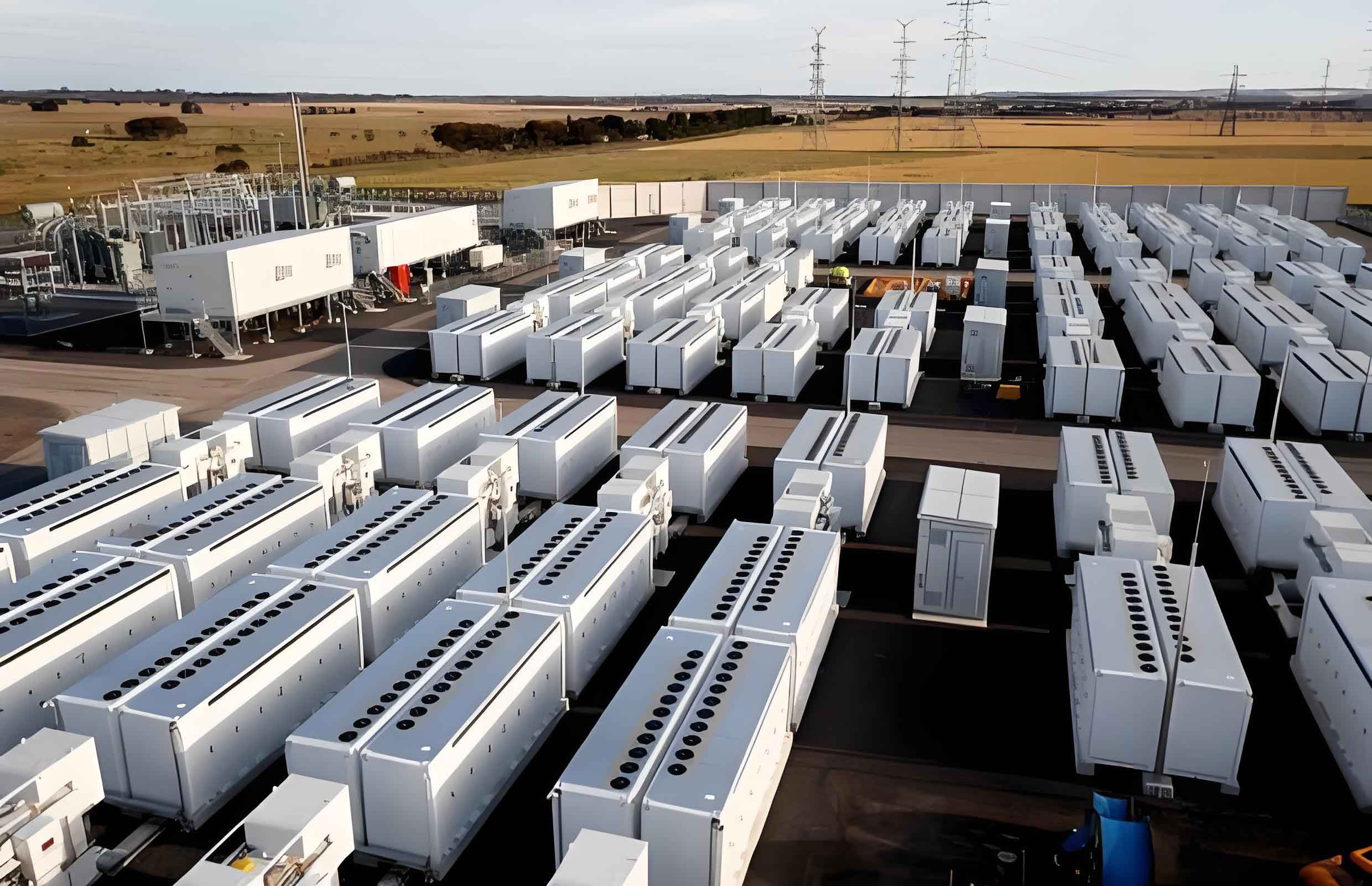
The typical structure of a battery energy storage system consists of the energy storage battery, the power conversion system (PCS), and the monitoring system. In DIgSILENT, I use a static generator as the grid interface for the BESS. The static generator is controlled by active current \(i_d\) and reactive current \(i_q\) in the d-q reference frame. The relationship between powers and currents is expressed as:
$$
\begin{aligned}
P &= u_d i_d + u_q i_q \\
Q &= u_q i_d – u_d i_q
\end{aligned}
$$
For balanced three-phase systems, the equations can be simplified to:
$$
P = u_d i_d, \qquad Q = -u_d i_q
$$
The overall BESS electromechanical transient model is shown in the following architecture: the outer power control loop, the frequency control loop, the charge/discharge control loop, the battery model, and the converter model. The converter is represented by a first-order inertia element:
$$
G_{cp}(s) = \frac{1}{1+T_{ip} s}
$$
$$
G_{cq}(s) = \frac{1}{1+T_{iq} s}
$$
where \(T_{ip}\) and \(T_{iq}\) are the current-loop time constants on the d and q axes, respectively.
2.2 Battery Modeling
The energy storage battery model is based on the typical discharge curve of a lead-acid battery. Considering the electromechanical transient time scale, I focus on the SOC range between 0.2 p.u. and 0.8 p.u., where the battery terminal voltage and internal resistance can be treated as constant. The SOC is calculated by:
$$
SOC(t) = SOC_{ini} – \frac{1}{3600 \cdot S_{BESS}} \int_0^t P_{BESS}(\tau)\, d\tau
$$
where \(SOC_{ini}\) is the initial SOC, \(P_{BESS}\) is the output active power of the energy storage battery, and \(S_{BESS}\) is the rated apparent power of the BESS.
2.3 Controller Design
The frequency controller adopts droop control with a dead band to avoid frequent charging/discharging. The active power command is given by:
$$
dp_{ref} = K_{droop}(f_{ref} – f_e)
$$
where \(K_{droop}\) is the droop coefficient, \(f_{ref}\) is the reference frequency, and \(f_e\) is the measured frequency. The power controller consists of an active power deviation control loop and a constant voltage control loop. The active power loop uses a PI controller to generate the d-axis current reference:
$$
dp = dp_{ref} + P_{ref} – P_e
$$
$$
i_{d\_ref\_in} = \left(K_p + \frac{1}{s T_p}\right) dp
$$
Similarly, the voltage control loop generates the q-axis current reference:
$$
i_{q\_ref\_in} = \left(K_q + \frac{1}{s T_q}\right) dv
$$
where \(dv = V_{ref} – V_e\) is the voltage error, \(K_p\), \(T_p\), \(K_q\), \(T_q\) are the PI parameters.
The charge/discharge controller limits the current reference values based on SOC constraints and converter current limits. When the SOC is outside the range [0.2 p.u., 0.8 p.u.], the d-axis current reference is set to zero. The current limiting strategy is designed with active power priority. However, when the bus voltage drops by more than 0.1 p.u., the d-q axis currents are swapped to give reactive power priority for fault ride-through capability.
2.4 Simulation Verification
I built a single-machine two-load system in DIgSILENT to verify the proposed BESS model. The system parameters are summarized in the following table:
| Component | Active Power (MW) | Reactive Power (Mvar) |
|---|---|---|
| Generator G1 | 50 | 20 |
| Load A | 10 | 2 |
| Load B | 50 | 10 |
The BESS controller parameters are listed below:
| Parameter | \(K_p\) | \(T_p\) | \(T_{ip}\) | \(K_q\) | \(T_q\) | \(T_{iq}\) | \(K_{droop}\) |
|---|---|---|---|---|---|---|---|
| Value | 1 | 0.1 | 0.01 | 1 | 0.1 | 0.01 | 0.04 |
Two disturbance scenarios were simulated: a single-phase ground fault at the generator outlet bus and a load step change. The simulation results show that the BESS responds correctly to grid disturbances. The energy storage battery provides active and reactive power support immediately after the fault, and the output gradually returns to zero as the system stabilizes. The frequency recovery time is shortened from 8.83 s to 3.07 s after BESS integration, although the frequency nadir slightly degrades from 49.147 Hz to 49.139 Hz due to overshoot in active power output. The voltage nadir improves from 0.395 p.u. to 0.420 p.u. The SOC curve accurately tracks the active power output of the energy storage battery. Therefore, the proposed BESS electromechanical transient model effectively reflects the dynamic response of the energy storage battery system and is suitable for power system transient stability analysis.
3. Parameter Identification Strategy for BESS Controller
3.1 Sensitivity Analysis
Parameter identifiability is essential for successful identification. I define the trajectory sensitivity of the output variable \(y_i\) with respect to parameter \(\theta_j\) as:
$$
S_{\theta_j}^{y_i}(t) = \frac{\partial y_i(t,\boldsymbol{\theta})}{\partial \theta_j}
\approx \frac{y_i(t, \theta_j + \Delta \theta_j, \boldsymbol{\theta}_{-j}) – y_i(t, \theta_j, \boldsymbol{\theta}_{-j})}{\Delta \theta_j}
$$
I performed trajectory sensitivity analysis for the BESS controller parameters \(K_p\), \(T_p\), \(T_{ip}\), \(K_q\), \(T_q\), and \(T_{iq}\). The candidate observation quantities are the active power output \(P\), reactive power output \(Q\), and terminal voltage \(V\). The disturbance scenarios are a three-phase short circuit at the point of common coupling and a step change in active power and voltage references.
The sensitivity results show that:
- When using active power as the observation, d-axis parameters have significantly higher sensitivity than q-axis parameters.
- When using reactive power as the observation, q-axis parameters have significantly higher sensitivity than d-axis parameters.
- When using voltage as the observation, the overall sensitivity is much lower than that of active and reactive power, making voltage unsuitable for parameter identification.
Therefore, I selected active power and reactive power as the observation quantities for the identification process.
3.2 Parameter Identification Framework in DIgSILENT
DIgSILENT provides a built-in parameter identification tool that compares measured and simulated transient trajectories. The identification principle is shown in the following process:
- Measurement files provide the measured active and reactive power data.
- The component model (BESS) receives excitation signals and outputs simulated data.
- The comparator calculates the objective function based on the sum of squared errors between measured and simulated data.
- The optimizer adjusts the controller parameters to minimize the objective function.
The objective function is defined as:
$$
F_p = \sum_{i=1}^{n} \omega_i |M_i – S_i|^p
$$
The default value of \(p\) is 2, and the weight factor \(\omega_i\) is set to 1 by default. For the BESS parameter identification, I define the composite objective function:
$$
F = \sum_{i=1}^{n} \omega_1 |M_{1,i} – S_{1,i}|^2 + \sum_{i=1}^{n} \omega_2 |M_{2,i} – S_{2,i}|^2
$$
where \(M_{1,i}\) and \(S_{1,i}\) are the measured and simulated active power data, and \(M_{2,i}\) and \(S_{2,i}\) are the measured and simulated reactive power data, respectively.
I implemented the parameter identification framework in DIgSILENT using the following modules:
ElmFile/ Measurement File: stores the measured data in a CSV-like format.ElmDsl/ Component Model: the BESS electromechanical transient model.ElmCompare/ Comparator: calculates the difference between simulated and measured data.Comldent/ Optimizer: modifies the parameters using an optimization algorithm.
I chose the quasi-Newton method for the identification because it is less sensitive to initial parameter values and converges quickly. The overall identification procedure is as follows:
| Step | Action |
|---|---|
| 1 | Select disturbance scenario (short circuit or step change) |
| 2 | Run a transient simulation and record the measured active and reactive power trajectories |
| 3 | Initialize the controller parameters in DIgSILENT |
| 4 | Run the identification optimizer to minimize the objective function |
| 5 | Validate the identified parameters by comparing simulated and measured curves |
3.3 Simulation Results under Three-Phase Short Circuit
The identification test system is a single-machine infinite-bus system with the BESS. The true values and initial values of the controller parameters are listed in the following table:
| Parameter | Initial Value | True Value | Range |
|---|---|---|---|
| \(K_p\) | 1 | 3 | [1,20] |
| \(T_p\) | 0.1 | 0.02 | [0.0001,1] |
| \(T_{ip}\) | 0.01 | 0.05 | [0.0001,1] |
| \(K_q\) | 1 | 3 | [1,20] |
| \(T_q\) | 0.1 | 0.02 | [0.0001,1] |
| \(T_{iq}\) | 0.01 | 0.05 | [0.0001,1] |
After 200 iterations of the quasi-Newton method, the objective function decreased from \(7.07 \times 10^{-2}\) to \(5.37 \times 10^{-4}\). The identification results are:
| Parameter | \(K_p\) | \(T_p\) | \(T_{ip}\) | \(K_q\) | \(T_q\) | \(T_{iq}\) |
|---|---|---|---|---|---|---|
| True Value | 3 | 0.02 | 0.05 | 3 | 0.02 | 0.05 |
| Identified Value | 2.8434 | 0.0196 | 0.0473 | 3.0124 | 0.014 | 0.0498 |
| Error (%) | -5.22 | -2.00 | -5.40 | 0.41 | -30 | -0.40 |
The identification accuracy is high for \(K_q\) and \(T_{iq}\), moderate for \(T_p\), \(K_p\), and \(T_{ip}\), and poor for \(T_q\). This is because the trajectory sensitivity of \(T_q\) is very low. However, the overall fitting of active power, reactive power, voltage, and current curves is excellent, indicating that the identified parameters can accurately reproduce the transient behavior of the energy storage battery system.
3.4 Simulation Results under Step Change Disturbance
For the step change scenario, the active power reference and voltage reference are changed at \(t=0.1\) s and \(t=0.2\) s. The objective function decreased from \(6.52 \times 10^{-2}\) to \(3.8 \times 10^{-5}\). The identification results are:
| Parameter | \(K_p\) | \(T_p\) | \(T_{ip}\) | \(K_q\) | \(T_q\) | \(T_{iq}\) |
|---|---|---|---|---|---|---|
| True Value | 3 | 0.02 | 0.05 | 3 | 0.02 | 0.05 |
| Identified Value | 3.0133 | 0.0199 | 0.0505 | 3.1434 | 0.0124 | 0.0479 |
| Error (%) | 0.44 | -0.50 | 1.00 | 4.78 | -38 | -4.20 |
Under the step change disturbance, the d-axis parameters are identified with very high accuracy, while the q-axis parameters show slightly larger errors. Again, the fitting of the dynamic response curves is very good. Therefore, the proposed parameter identification strategy is effective for both fault disturbances and manual step changes. The results confirm that parameters with higher trajectory sensitivity are easier to identify accurately. For practical applications, one can choose the disturbance type that provides the highest sensitivity for the parameters of interest.
4. Control Parameter Optimization for Transient Stability Improvement
4.1 Qualitative Analysis of Transient Stability
I analyzed the influence of the energy storage battery on the transient stability of a synchronous generator using a single-machine infinite-bus system with a BESS. The generator is represented by a transient electromotive force and reactance, while the BESS is modeled as a controllable power source. The electromagnetic torque increment \(\Delta M_e\) and the generator power increment \(\Delta P_G\) can be expressed as:
$$
\Delta M_e = k_{e1} \Delta \delta_1 + k_{e2} \Delta P_S
$$
$$
\Delta P_G = k_{d1} \Delta \delta_1 + k_{d2} \Delta P_S
$$
Using the simplified first-order inertia model of the BESS converter, the BESS active power output is:
$$
\Delta P_S = \frac{k_{e1}}{1 + T s} \Delta P_G
$$
Substituting and simplifying yields the synchronizing torque coefficient \(K_S\) and damping torque coefficient \(K_D\):
$$
K_S = k_{c1} + \frac{k_{c2} k_{e1} k_{d1}}{1 + k_{e1} k_{d2}}
$$
$$
K_D = \frac{k_{c2} k_{e1} k_{d1} T}{(1 + k_{e1} k_{d2})^2}
$$
From these equations, the BESS active power regulation coefficient \(k_{e1}\) affects both the synchronizing and damping torque of the generator. Therefore, proper tuning of the BESS controller parameters can improve the transient stability margin of the power system.
The optimization objective is to minimize the sum of squared errors (SSE) of the generator rotor angles after a fault:
$$
F_{G\_SSE} = \sum_{m=1}^{n} \sum_{i=1}^{k} \left( t_{m,i} – a \right)^2
$$
where \(t_{m,i}\) is the rotor angle of generator \(m\) at time \(i\), \(a\) is the steady-state rotor angle, \(n\) is the number of generators, and \(k\) is the number of sampled points. To avoid voltage degradation, I added a constraint on the bus voltage SSE:
$$
F_{V\_SSE} = \sum_{j=1}^{x} \left( l_{no,j} – b \right)^2 – \sum_{j=1}^{x} \left( l_{with,j} – b \right)^2 \geq 0
$$
where \(l_{no,j}\) and \(l_{with,j}\) are the voltage trajectories before and after BESS integration at the central bus, and \(b\) is the steady-state voltage. This constraint ensures that the optimized parameters do not worsen the voltage recovery performance.
4.2 DIgSILENT-Python Co-Simulation Framework
DIgSILENT has a built-in optimization module, but it can only optimize components with measurement functions. Generator rotor angles and damping coefficients cannot be directly used as optimization targets. To solve this problem, I developed a co-simulation framework that couples DIgSILENT and Python. The framework is illustrated in the following flow:
- DIgSILENT executes the transient simulation and exports the result files.
- Python reads the simulation results, computes the fitness function, and runs the particle swarm optimization (PSO) algorithm.
- Python sends the new parameter values to DIgSILENT via the remote scripting interface.
- DIgSILENT updates the controller parameters and repeats the simulation until the stopping criterion is met.
The key functions of the co-simulation are implemented using the DIgSILENT PowerFactory Python API. The automation simulation commands include:
- Load the active study case using
GetApplication. - Execute power flow calculation with
ComLdf. - Initialize transient simulation conditions with
ComLnc. - Run the electromechanical transient simulation with
Comsim. - Export results to CSV files using
ComResandiopt_exp=6. - Read or set controller parameters using
GetAttributeandSetAttribute.
The PSO algorithm parameters are shown below:
| PSO Parameter | Value |
|---|---|
| Population size \(P\) | 20 |
| Maximum iterations \(I\) | 200 |
| Acceleration coefficient \(c_1\) | 1.0 |
| Acceleration coefficient \(c_2\) | 1.4 |
| Inertia weight \(\omega\) | 0.7 |
| Number of optimized parameters | 7 |
4.3 Simulation Setup on IEEE 9-Bus System
I modified the standard IEEE 9-bus system by adding a battery energy storage system at bus 4. The system consists of three synchronous generators, three loads, and a BESS. The generator and load data are summarized as follows:
| Component | Active Power (MW) | Reactive Power (Mvar) |
|---|---|---|
| G1 | 71.6 | 27 |
| G2 | 163 | 6.7 |
| G3 | 85 | -10.9 |
| Load A | 125 | 50 |
| Load B | 90 | 30 |
| Load C | 100 | 35 |
The initial measured parameters of the BESS controller are taken from practical data. The optimization variables are \(K_p\), \(T_p\), \(T_{ip}\), \(K_q\), \(T_q\), \(T_{iq}\), and \(K_{droop}\). The ranges are given in the following table:
| Parameter | Measured Value | Optimized Value | Range |
|---|---|---|---|
| \(K_p\) | 2 | 4.824 | [1,20] |
| \(T_p\) | 0.01 | 0.020 | [0.0001,1] |
| \(T_{ip}\) | 0.01 | 0.005 | [0.0001,1] |
| \(K_q\) | 2 | 5.012 | [1,20] |
| \(T_q\) | 0.01 | 0.014 | [0.0001,1] |
| \(T_{iq}\) | 0.01 | 0.005 | [0.0001,1] |
| \(K_{droop}\) | 0.004 | 0.011 | [0.002,0.04] |
Under a three-phase short circuit at line 5-7, I compared three cases: no BESS, BESS with measured parameters, and BESS with optimized parameters. The rotor angle curves of generator G2 and G3 clearly show that the BESS reduces the first swing amplitude and damps subsequent oscillations. The objective function \(F_{G\_SSE}\) decreased from 348.591 to 323.442, an improvement of 7.21%. The central bus voltage SSE also improved from 1.273 (no BESS) and 1.259 (measured) to 1.237 (optimized).
| Case | G2 First Swing (deg) | G3 First Swing (deg) | \(F_{G\_SSE}\) (p.u.) | Bus 4 SSE (p.u.) |
|---|---|---|---|---|
| No BESS | 86.928 | 67.272 | 348.591 | 1.273 |
| Measured parameters | 85.825 | 65.079 | 348.591 | 1.259 |
| Optimized parameters | 85.180 | 64.235 | 323.442 | 1.237 |
4.4 Adaptability Verification of the Optimized Parameters
To verify that the optimized parameters are applicable to other disturbance scenarios, I performed two additional simulations: a load step change and a single-phase ground fault.
4.4.1 Load Step Change
At \(t=0.5\) s, load C is reduced by 80%, and restored at \(t=1.5\) s. The results show that the optimized parameters provide faster voltage recovery and smoother rotor angle oscillations compared to the measured parameters. The SSE indicators are listed in the following table:
| Indicator | No BESS | Measured Parameters | Optimized Parameters |
|---|---|---|---|
| G2 SSE (p.u.) | 82.728 | 72.512 | 70.098 |
| G3 SSE (p.u.) | 76.738 | 68.619 | 66.876 |
| Bus 4 SSE (p.u.) | 0.275 | 0.166 | 0.145 |
Compared to the measured parameters, the optimized parameters reduce the G2 SSE by 3.33% and the G3 SSE by 2.54%. The voltage SSE is also reduced by 12.65%. This confirms that the optimized parameters improve the transient stability for load step disturbances.
4.4.2 Single-Phase Ground Fault
At \(t=0.5\) s, a single-phase ground fault occurs at bus 9 and is cleared after 0.1 s. The SSE results are:
| Indicator | No BESS | Measured Parameters | Optimized Parameters |
|---|---|---|---|
| G2 SSE (p.u.) | 155.396 | 134.823 | 128.278 |
| G3 SSE (p.u.) | 142.427 | 129.703 | 125.758 |
| Bus 4 SSE (p.u.) | 1.172 | 1.137 | 1.122 |
The optimized parameters reduce the G2 SSE by 4.85% and the G3 SSE by 3.04% compared to the measured parameters. These results demonstrate that the parameters optimized under a three-phase short circuit are also effective for other fault types, confirming the robustness and adaptability of the proposed optimization framework.
5. Conclusion and Future Work
In this thesis, I conducted comprehensive research on the modeling, parameter identification, and control optimization of the battery energy storage system (energy storage battery). The main contributions and conclusions are as follows:
-
Electromechanical transient modeling: I established a simplified BESS electromechanical transient model that captures the essential dynamic behavior of the energy storage battery, the converter, and the control system. The model correctly represents the SOC dynamics and the converter current limits. Simulation results show that the BESS can provide effective frequency and voltage support during grid disturbances.
-
Parameter identification: I proposed a trajectory-sensitivity-based parameter identification strategy. The analysis shows that active power is a suitable observation for d-axis parameters, while reactive power is suitable for q-axis parameters. The identification framework implemented in DIgSILENT successfully identifies the controller parameters under both short-circuit faults and step changes. The accuracy of the identified parameters is consistent with the trajectory sensitivity analysis.
-
Control optimization: I developed a DIgSILENT-Python co-simulation framework using particle swarm optimization to tune the BESS controller parameters. The optimized parameters effectively reduce the generator first swing angle, damp power angle oscillations, and improve the voltage recovery at the central bus. The optimized parameters also perform well under different disturbance scenarios, confirming their adaptability.
There are some limitations in my current research. First, the fault ride-through control only considers reactive power priority and could be extended to more sophisticated high-low voltage ride-through strategies. Second, the parameter identification was tested only for two representative disturbance patterns, so the universality needs further validation with other disturbance types. Finally, the optimization algorithm is the standard PSO; more advanced or hybrid algorithms could be explored to improve convergence speed and solution quality. Future work will focus on these aspects to further enhance the performance of the energy storage battery system in real power system applications.