
1. Introduction
Driven by the global strategic goals of carbon peak and carbon neutrality, the transformation of energy systems has entered a substantive stage worldwide. The solar panel industry, as a key pillar of low-carbon energy transition, has experienced rapid development in recent years. By mid-2024, the total installed capacity of solar photovoltaic power generation had exceeded 712.93 GW. However, solar panels are predominantly deployed in harsh environmental conditions, making them susceptible to various defects such as cracks, stains, grid breakages, and hot spots, which severely impact power generation efficiency and system stability. Therefore, precise and efficient solar panel defect detection is of paramount importance for eliminating safety hazards, optimizing system performance, improving power generation efficiency, and reducing operation and maintenance costs.
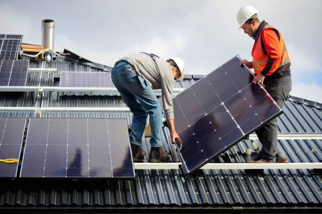
Traditional methods for solar panel defect detection, such as K-means clustering and support vector machine (SVM) based multi-feature fusion, have achieved certain progress in specific scenarios. However, these approaches generally suffer from high computational complexity and insufficient scene adaptability, making it difficult to meet the demands of large-scale inspection. In recent years, deep learning-based object detection algorithms have demonstrated remarkable performance in various computer vision tasks, including defect detection. Among these, convolutional neural network (CNN) based methods have gained significant traction in the solar panel inspection domain.
Deep learning algorithms for solar panel defect detection can be broadly categorized into two-stage and one-stage approaches, each offering distinct advantages in terms of detection accuracy and real-time performance. Two-stage methods, represented by the R-CNN family, typically achieve higher accuracy but at the cost of larger model sizes and higher computational complexity, making them challenging to deploy on embedded devices. One-stage methods, such as SSD and the YOLO series, have gained popularity due to their end-to-end training capability and superior inference speed, making them more suitable for real-time detection scenarios.
Among the YOLO family, YOLO11n represents the latest lightweight object detection algorithm, featuring innovative modules such as C3k2 and C2PSA, along with an end-to-end training strategy without non-maximum suppression (NMS). However, when applied to infrared solar panel defect detection from UAV platforms, several challenges persist: small target defects with blurred infrared features and insufficient resolution lead to missed detections; complex and diverse defect characteristics with multi-scale distribution make it difficult to simultaneously capture global panel features and local thermal anomalies; and the model’s parameter count and computational complexity remain relatively high for embedded deployment.
To address these challenges, we propose HBGF-YOLO, an improved object detection algorithm based on the YOLO11n framework. Our approach introduces three key innovations: First, we design Rep-HGNetV2, an efficient backbone network that integrates hierarchical gradient feature extraction with re-parameterized convolution techniques, enhancing feature extraction capability while reducing model complexity. Second, we construct a collaborative architecture combining a bidirectional feature pyramid network (BiFPN) with a global-local self-attention mechanism (GLSA) to effectively capture both global thermal distribution patterns and local detail features. Third, we employ a feature enhancement fusion module (FEFM) that achieves deep cross-layer feature fusion through dynamic weight adaptation, strengthening semantic information propagation for tiny defect regions.
2. Related Work
2.1 Solar Panel Defect Detection
Solar panel defect detection has been an active research area, with various approaches being explored. Traditional machine learning methods often rely on hand-crafted features and shallow classifiers, which struggle to generalize across different defect types and environmental conditions. Deep learning-based approaches have shown superior performance in automatically learning discriminative features from data. Two-stage detectors like Faster R-CNN have been applied to hot spot detection in solar panels, achieving high accuracy but with significant computational overhead. One-stage detectors, particularly the YOLO series, have been widely adopted for real-time solar panel inspection due to their balance between speed and accuracy.
2.2 Lightweight Object Detection
For UAV-based applications, lightweight object detection models are essential to meet the computational and memory constraints of embedded platforms. Various techniques have been explored to reduce model complexity while maintaining detection accuracy. These include depthwise separable convolutions, channel pruning, knowledge distillation, and neural architecture search. The YOLO series has evolved through multiple iterations, with each version introducing improvements in both efficiency and effectiveness. YOLO11n, as the latest lightweight variant, provides a solid foundation for further optimization in solar panel defect detection tasks.
3. HBGF-YOLO Methodology
In this section, we present the detailed architecture of the proposed HBGF-YOLO algorithm. Our approach introduces several key innovations to address the challenges of small target defect detection in UAV-based solar panel infrared imagery. The overall framework consists of three main components: the Rep-HGNetV2 backbone network, the BiFPN-GLSA feature fusion architecture, and the FEFM module for enhanced feature integration.
3.1 Rep-HGNetV2 Backbone Network
The backbone network is responsible for extracting hierarchical features from input images. In our design, we adopt HGNetV2, originally introduced in the RT-DETR model, as the base architecture. HGNetV2 employs a lightweight design philosophy, significantly reducing model parameters and computational complexity while maintaining competitive detection accuracy. The network comprises HGStem preprocessing layers and HGBlock data processing modules.
The HGStem module utilizes an efficient convolutional structure to achieve high-quality feature extraction at the initial input layer, enabling the network to obtain sufficient feature information with relatively low parameter and computational costs. The HGBlock, as the core component, employs a hierarchical data processing mechanism to capture features at different scales, achieving refined hierarchical processing of information and effectively enhancing the network’s sensitivity to solar panel defect details.
A critical component of HGNetV2 is the use of depthwise separable convolution (DWConv). Compared to standard convolution, DWConv offers significant advantages in terms of both parameter count and computational complexity. Given an input feature map with height H, width W, and input channels Cin, a convolution kernel size of K×K, and output channels Cout, the parameter count P and computational cost F for standard convolution are:
$$P = C_{in} \cdot C_{out} \cdot K \cdot K$$
$$F = C_{in} \cdot C_{out} \cdot W \cdot H \cdot K \cdot K$$
For depthwise separable convolution, the parameter count PDW and computational cost FDW are:
$$P_{DW} = C_{in} \cdot K \cdot K + C_{in} \cdot C_{out}$$
$$F_{DW} = C_{in} \cdot W \cdot H \cdot K \cdot K + C_{in} \cdot C_{out} \cdot W \cdot H$$
From these equations, we can derive the ratio:
$$\frac{P_{DW}}{P} = \frac{F_{DW}}{F} = \frac{1}{C_{out}} + \frac{1}{K^2}$$
This demonstrates that DWConv achieves a parameter and computational reduction by a factor of 1/Cout + 1/K2, which is the fundamental reason for the lightweight nature of HGNetV2.
To further optimize network performance, we introduce re-parameterized convolution (RepConv) into the HGBlock structure. During the training phase, RepConv employs a multi-branch architecture that parallelly fuses three paths: a 3×3 convolution for local detail extraction, a 1×1 convolution for channel interaction enhancement, and a batch normalization (BN) branch for preserving feature distribution. This multi-branch design fully exploits the diverse representational capacity of the data. During inference, the weights and BN parameters from all three branches are integrated into a single 3×3 convolution kernel, where the 1×1 convolution is expanded through zero-padding and BN parameters are merged into weights and biases. This results in a parameter count equivalent to standard convolution while inheriting the feature fusion advantages of multi-branch training.
3.2 BiFPN Feature Fusion Network
Solar panel defects exhibit complex and diverse characteristics with multi-scale distributions. The original YOLO11n feature fusion mechanism, which relies on simple concatenation operations, cannot effectively integrate feature information from different depth levels, limiting detection accuracy. To address this, we adopt the BiFPN architecture from the EfficientDet algorithm to optimize the feature fusion mechanism.
BiFPN implements bidirectional cross-scale connections with weighted feature fusion, effectively promoting top-down propagation of high-level semantic features and bottom-up integration of low-level fine spatial features. By simultaneously considering features at different scales, BiFPN leverages high-level features for global recognition and low-level features for detail preservation when processing both large-area thermal distributions and small-scale thermal anomalies. Compared to the original PANet structure in YOLO11n, BiFPN strengthens both same-level and cross-level feature fusion through cross-connection layers, enhancing the model’s detection accuracy for multi-scale solar panel defects.
3.3 Global-Local Self-Attention Mechanism
In infrared image feature fusion, small targets often exhibit low distinguishability from the background, and the lack of a dynamic feature balancing mechanism causes small target features to be weakened, limiting detection accuracy. We introduce the GLSA mechanism between the Rep-HGNetV2 backbone and BiFPN to address this issue.
GLSA receives feature maps extracted by Rep-HGNetV2 and performs semantic-level甄别 and enhancement. By reallocating weights based on the global semantic importance of features, GLSA highlights target features while suppressing background interference. This preprocessing enables BiFPN to operate on more precise and discriminative features during the fusion stage, better integrating multi-scale information for both large-scale features and small-scale details.
The GLSA module consists of two complementary branches: Local Spatial Attention (LSA) focuses on pixel-level details of defect regions, enhancing sensitivity to minute defect features; Global Spatial Attention (GSA) models the overall structural semantics of solar panels, suppressing repetitive texture and noise interference. Through cross-scale fusion of LSA and GSA, the module preserves local fine features of defects while utilizing global contextual information to strengthen feature discriminability, effectively balancing detail capture and background suppression capabilities.
The computational process of GLSA can be formulated as follows. Given an input feature X of dimension (C, H, W), channel splitting is first performed to obtain X0 and X1:
$$X_0, X_1 = \text{split}(X)$$
The GSA branch computes attention weights through:
$$\text{Att}_G(X_0) = \text{Softmax}(\text{transpose}(\text{Conv}_{1\times1}(X_0)))$$
$$\text{GSA}(X_0) = \text{MLP}(\text{Att}_G(X_0) \otimes X_0) + X_0$$
The LSA branch computes attention weights through:
$$\text{Att}_L(X_1) = \text{Sigmoid}(\text{Conv}_{1\times1}(\text{DWConv}_{3\times3}(\text{Conv}_{1\times1}(X_1)))) \times 3 + X_1$$
$$\text{LSA}(X_1) = \text{Att}_L(X_1) \odot X_1 + X_1$$
The final output is obtained by concatenating the GSA and LSA outputs along the channel dimension and applying 1×1 convolution for dimension reduction:
$$Y = \text{Conv}_{1\times1}(\text{Concat}(\text{GSA}(X_0), \text{LSA}(X_1)))$$
3.4 Feature Enhancement Fusion Module
The feature fusion in the original YOLO11n primarily relies on simple concatenation operations, which apply average weighting to information from different feature maps. This approach cannot dynamically adapt to the importance and relevance of different feature maps, limiting the model’s detection accuracy and generalization capability. To address this, we introduce the FEFM for adaptive weighted fusion of different feature maps, dynamically learning the importance and relevance of different feature sources to more effectively integrate multi-source feature information.
FEFM employs an edge-semantic two-stage cascaded optimization mechanism to enhance feature discriminability. First, shallow high-resolution edge features are utilized to enhance local detail representation, highlighting boundary responses of minute defects. Subsequently, deep semantic features are introduced to dynamically calibrate fusion weights, suppressing background noise while strengthening defect region features.
Given a low-level feature map FL and a high-level feature map (either high-level feature FH or edge feature FE), the FEFM process begins by applying Coordinate Attention (CA) to enhance spatial information in the low-level features:
$$F’_L = \text{CA}(F_L)$$
Context Modeling (CM) is then applied to extract channel weights MCM from the edge features:
$$M_{CM} = \text{CM}(F_E)$$
The optimized features are obtained through element-wise multiplication:
$$F”_L = M_{CM} \otimes F’_L$$
Finally, the enhanced low-level features are concatenated with the edge features:
$$F_O = \text{Concat}[F”_L, F_E]$$
The Coordinate Attention mechanism enhances defect region localization through direction-aware and position-sensitive feature modeling. It first performs global average pooling along the height and width dimensions to generate vertical and horizontal response maps. The vertical response map zh(c) and horizontal response map zw(c) are computed as:
$$z_h(c) = \frac{1}{W} \sum_{0 \leq i \leq W} x_c(h, i)$$
$$z_w(c) = \frac{1}{H} \sum_{j} x_c(j, w)$$
These are then concatenated along the channel dimension and processed through a 1×1 convolution to generate spatial attention weights:
$$f = \delta(\text{Conv}_{1\times1}([z_h, z_w]))$$
$$g_h = \sigma(\text{Conv}_h(f))$$
$$g_w = \sigma(\text{Conv}_w(f))$$
$$F_{out} = x \times g_h \times g_w$$
The Context Modeling module captures contextual features by first generating attention maps through 1×1 convolution and Softmax activation, then performing weighted integration of features across spatial positions through matrix operations:
$$F_{CM}^{out} = I * (z(\text{Conv}_{1\times1}(I)))$$
where I represents the input feature map, z represents Softmax activation, and * denotes matrix multiplication.
4. Experimental Setup
4.1 Dataset
We constructed a specialized solar panel defect detection dataset using infrared images captured by a DJI M300 RTK UAV equipped with a FLIR XT2 infrared camera. The dataset comprises 3,225 thermal imaging images covering five categories: large-area hot spots (dmjrb), single hot spots (dyrb), abnormal low temperature (ycdw), diode short circuit (ejgdl), and normal state (zc). Each image contains multiple solar panels, and each individual panel was manually annotated using the Labelimg tool to ensure accurate recording of defect status.
To ensure reliable experimental results, the dataset was split into training, validation, and test sets in a 7:2:1 ratio. Data augmentation techniques including random rotation, mirror flipping, and noise addition were applied to expand the training set to 6,773 images, enhancing model generalization performance. The dataset statistics are summarized in the following table:
| Label | dmjrb | dyrb | ycdw | ejgdl | zc |
|---|---|---|---|---|---|
| Counts | 1,373 | 1,678 | 1,125 | 1,049 | 4,870 |
4.2 Implementation Details
All experiments were conducted on a high-performance computing platform. The hardware configuration, software environment, and training parameters are specified in the following tables:
| Environment | Specification |
|---|---|
| Operating system | Windows 11 |
| Processor | Intel Core i5-12400F |
| Programming language | Python 3.9 |
| Deep learning framework | PyTorch 1.12 |
| GPU | RTX 4060Ti |
| Parameter | Value |
|---|---|
| Input size | 640×640 |
| Batch size | 16 |
| Epoch | 300 |
| Optimizer | SGD |
| Initial learning rate | 0.01 |
4.3 Evaluation Metrics
We employed comprehensive evaluation metrics to assess model performance, including precision (P), recall (R), mean average precision (mAP), parameter count (Params), and floating-point operations (FLOPs):
$$P = \frac{N_{TP}}{N_{TP} + N_{FP}}$$
$$R = \frac{N_{TP}}{N_{TP} + N_{FN}}$$
$$P_{AP} = \int_{0}^{1} P(R) dr$$
$$P_{mAP} = \frac{1}{n} \sum_{i=1}^{n} P_{AP}$$
where NTP represents the number of true positive samples correctly classified, NFP represents false positives, and NFN represents false negatives.
5. Experimental Results and Analysis
5.1 Backbone Network Performance Analysis
To validate the effectiveness of introducing HGNetV2 as the backbone network for solar panel defect detection, we conducted comparative experiments with other lightweight backbone networks. The results are presented in the following table:
| Base model | Backbone network | P (%) | R (%) | PmAP50 (%) | PmAP50-95 (%) | Params (106) | FLOPs (109) |
|---|---|---|---|---|---|---|---|
| YOLO11n | BottleNeck | 84.7 | 78.3 | 83.4 | 70.9 | 2.6 | 6.3 |
| YOLO11n | ShuffleNetV2 | 80.3 | 73.8 | 78.7 | 66.9 | 1.6 | 3.6 |
| YOLO11n | EfficientViT | 84.0 | 77.1 | 80.7 | 68.7 | 3.8 | 8.1 |
| YOLO11n | MobileNetV4 | 84.1 | 77.3 | 80.9 | 68.7 | 5.4 | 21.0 |
| YOLO11n | StartNet | 85.6 | 76.5 | 81.2 | 68.9 | 1.9 | 5.0 |
| YOLO11n | FasterNet | 85.8 | 80.2 | 83.1 | 70.5 | 3.9 | 9.2 |
| YOLO11n | HGNetV2 | 84.6 | 77.5 | 82.9 | 70.8 | 2.2 | 5.9 |
| YOLO11n | Rep-HGNetV2 | 84.5 | 81.2 | 84.2 | 71.9 | 2.1 | 5.7 |
The experimental results demonstrate that HGNetV2 achieves competitive detection accuracy while significantly reducing parameter count and computational complexity compared to the original BottleNeck backbone. When RepConv is introduced into HGNetV2, the PmAP50 and PmAP50-95 improve by 1.3 and 1.1 percentage points respectively, confirming that RepConv enhances the model’s ability to identify target defects. Compared to the original model, Rep-HGNetV2 improves PmAP50 and PmAP50-95 by 0.8 and 1.0 percentage points respectively, while reducing parameters by 19.2% and computational complexity by 9.5%.
5.2 Feature Fusion Performance Analysis
To evaluate the effectiveness of different feature fusion networks, we conducted comparative experiments with Rep-HGNetV2 as the backbone. The results are shown in the following table:
| Base model | Neck network | P (%) | R (%) | PmAP50 (%) | PmAP50-95 (%) | Params (106) | FLOPs (109) |
|---|---|---|---|---|---|---|---|
| YOLO11n+Rep-HGNetV2 | PANet | 84.5 | 81.2 | 84.2 | 71.9 | 2.1 | 5.7 |
| YOLO11n+Rep-HGNetV2 | BiFPN | 85.1 | 81.5 | 84.7 | 72.8 | 1.8 | 6.1 |
The results indicate that BiFPN achieves superior detection performance compared to PANet, with PmAP50 and PmAP50-95 reaching 84.7% and 72.8% respectively. Although BiFPN has slightly higher computational complexity, its accuracy improvements validate its effectiveness for solar panel defect detection tasks.
5.3 Attention Mechanism Comparison
To address the challenge of small-scale defect features being easily overlooked, we introduced GLSA to simultaneously capture global contextual information and local detail features. Comparative experiments with other attention mechanisms were conducted, with results presented in the following table:
| Base model | Attention | P (%) | R (%) | PmAP50 (%) | PmAP50-95 (%) | Params (106) | FLOPs (109) |
|---|---|---|---|---|---|---|---|
| YOLO11n+Rep-HGNetV2+BiFPN | CAFM | 82.4 | 80.3 | 83.7 | 71.0 | 2.3 | 8.4 |
| YOLO11n+Rep-HGNetV2+BiFPN | CPCA | 83.5 | 79.2 | 84.5 | 71.7 | 1.8 | 7.3 |
| YOLO11n+Rep-HGNetV2+BiFPN | MLCA | 85.9 | 79.9 | 84.9 | 72.3 | 1.5 | 5.6 |
| YOLO11n+Rep-HGNetV2+BiFPN | SegNext | 84.2 | 82.2 | 85.1 | 72.3 | 1.7 | 6.4 |
| YOLO11n+Rep-HGNetV2+BiFPN | GLSA | 86.2 | 82.6 | 85.2 | 72.6 | 1.7 | 6.2 |
The experimental results demonstrate that GLSA achieves the highest precision, recall, and detection accuracy among all compared attention mechanisms. While its parameter count and computational complexity are slightly higher than MLCA, GLSA offers the best overall balance between accuracy and efficiency, making it the most suitable choice for solar panel defect detection.
5.4 Ablation Study
To comprehensively evaluate the effectiveness of each proposed improvement, we conducted a systematic ablation study by gradually introducing each module and analyzing its impact on detection performance. The results are summarized in the following table:
| RH | BF | GL | FE | P (%) | R (%) | PmAP50 (%) | PmAP50-95 (%) | Params (106) | FLOPs (109) |
|---|---|---|---|---|---|---|---|---|---|
| 84.7 | 78.3 | 83.4 | 70.9 | 2.6 | 6.3 | ||||
| √ | 84.5 | 81.2 | 84.2 | 71.9 | 2.1 | 5.7 | |||
| √ | √ | 85.1 | 81.5 | 84.7 | 72.8 | 1.8 | 6.1 | ||
| √ | √ | √ | 86.2 | 82.6 | 85.2 | 72.6 | 1.7 | 6.2 | |
| √ | √ | √ | √ | 87.3 | 81.7 | 85.5 | 73.2 | 1.6 | 5.8 |
Note: RH = Rep-HGNetV2, BF = BiFPN, GL = GLSA, FE = FEFM.
The ablation study reveals that each module contributes positively to model performance. The complete HBGF-YOLO model achieves precision of 87.3% and recall of 81.7%, with PmAP50 and PmAP50-95 reaching 85.5% and 73.2% respectively. Compared to the baseline YOLO11n, our improved model shows significant improvements of 2.6 percentage points in precision, 3.4 percentage points in recall, 2.1 percentage points in PmAP50, and 2.3 percentage points in PmAP50-95, while reducing parameters by 38.5% and computational complexity by 7.9%.
5.5 Comparison with State-of-the-Art Methods
To validate the superiority of our proposed HBGF-YOLO, we conducted comprehensive comparisons with state-of-the-art object detection algorithms on our solar panel dataset. The quantitative results are presented in the following table:
| Model | P (%) | R (%) | PmAP50 (%) | PmAP50-95 (%) | Params (106) | FLOPs (109) |
|---|---|---|---|---|---|---|
| Faster R-CNN | 71.2 | 70.9 | 74.3 | 61.8 | 43.6 | 207.0 |
| SSD | 65.8 | 68.0 | 68.7 | 59.5 | 25.2 | 34.3 |
| ShuffleNet v2 | 80.3 | 73.8 | 78.7 | 66.9 | 1.6 | 3.6 |
| MobileNet v4 | 84.1 | 77.3 | 80.9 | 68.7 | 5.4 | 21.0 |
| YOLOv3-tiny+ | 80.5 | 77.2 | 78.7 | 68.6 | 9.4 | 15.7 |
| YOLOv5n | 77.7 | 76.2 | 78.5 | 65.9 | 2.1 | 5.8 |
| YOLOv5n+ | 78.2 | 76.0 | 79.1 | 66.7 | 13.2 | 24.3 |
| YOLOv5sm+ | 81.6 | 79.8 | 81.3 | 69.7 | 17.9 | 38.6 |
| YOLOv8n | 79.1 | 76.8 | 79.3 | 67.1 | 2.7 | 6.8 |
| LS-YOLO | 85.4 | 80.2 | 83.7 | 72.1 | 1.8 | 23.8 |
| YOLOv10n | 80.1 | 79.9 | 81.4 | 70.1 | 2.3 | 6.5 |
| YOLO11n | 84.7 | 78.3 | 83.4 | 70.9 | 2.6 | 6.3 |
| HBGF-YOLO | 87.3 | 81.7 | 85.5 | 73.2 | 1.6 | 5.8 |
The experimental results clearly demonstrate that HBGF-YOLO achieves the best overall performance among all compared methods. Our model achieves the highest precision (87.3%), recall (81.7%), PmAP50 (85.5%), and PmAP50-95 (73.2%) while maintaining the lowest parameter count (1.6 × 10⁶) and competitive computational complexity (5.8 × 10⁹ FLOPs). Compared to the baseline YOLO11n, HBGF-YOLO shows consistent improvements across all evaluation metrics while significantly reducing model size and computational requirements.
When compared to other lightweight detectors specifically designed for small target detection, such as LS-YOLO and YOLOv5n+, our method achieves superior accuracy with substantially lower computational costs. This demonstrates the effectiveness of our architectural innovations for solar panel defect detection in UAV-based infrared imagery.
5.6 Generalization Performance on MS COCO
To validate the generalization capability of our proposed HBGF-YOLO across different scenarios and datasets, we conducted comparative experiments on the MS COCO benchmark dataset. All models were trained using identical parameter settings, and the results are presented in the following table:
| Model | PmAP50-95 (%) | Params (106) | FLOPs (109) |
|---|---|---|---|
| Faster R-CNN | 36.4 | 42.1 | 207.0 |
| SSD | 25.1 | 27.4 | 33.6 |
| YOLOv5n | 28.0 | 1.9 | 4.5 |
| YOLOv7-tiny | 37.4 | 6.2 | 13.7 |
| YOLOv8n | 37.3 | 3.2 | 8.7 |
| YOLOv9t | 27.5 | 4.5 | 10.5 |
| YOLOv10n | 29.8 | 3.5 | 9.2 |
| YOLO11n | 39.5 | 2.6 | 6.5 |
| HBGF-YOLO | 40.3 | 1.7 | 5.9 |
The results on MS COCO demonstrate that HBGF-YOLO achieves the highest PmAP50-95 of 40.3% while maintaining the lowest parameter count (1.7 × 10⁶) and competitive computational complexity (5.9 × 10⁹ FLOPs). This confirms that our proposed architectural improvements are not specific to solar panel defect detection but generalize well to general object detection tasks. The superior performance on MS COCO, which contains diverse object categories at various scales, further validates the robustness and versatility of the HBGF-YOLO framework.
5.7 Feature Visualization and Analysis
To gain deeper insights into the effectiveness of our proposed modules, we conducted feature visualization analysis using heatmap representations. The introduction of GLSA significantly enhances the model’s focus on small target regions, with the red thermal response areas expanding and more accurately aligning with actual defect locations. This demonstrates that the global attention mechanism effectively localizes small targets by integrating scene contextual information, while the local attention mechanism enhances target-background contrast through detail strengthening.
Visual comparison between the baseline YOLO11n and HBGF-YOLO detection results reveals that our improved algorithm not only identifies more defects but also achieves higher confidence scores. This is particularly evident for small and subtle defects that are easily missed by the baseline model. The enhanced detection capability is attributed to the synergistic effect of all three proposed components: Rep-HGNetV2 provides efficient feature extraction, BiFPN-GLSA enables comprehensive multi-scale and contextual feature capture, and FEFM achieves deep adaptive feature fusion.
6. Discussion
6.1 Computational Efficiency Analysis
One of the primary challenges in UAV-based solar panel inspection is the limited computational resources available on embedded platforms. Our HBGF-YOLO model addresses this challenge through several design choices that collectively reduce computational requirements while maintaining high detection accuracy. The Rep-HGNetV2 backbone achieves significant parameter reduction through the combination of HGNetV2’s lightweight architecture and RepConv’s re-parameterization technique. The BiFPN optimizes feature fusion by reducing redundant connections while maintaining bidirectional information flow. The GLSA mechanism employs channel splitting to reduce computational overhead while preserving both global and local attention capabilities.
The overall computational efficiency of HBGF-YOLO makes it particularly suitable for real-time deployment on UAV platforms. With only 1.6 × 10⁶ parameters and 5.8 × 10⁹ FLOPs, our model can achieve high-speed inference on resource-constrained devices while maintaining superior detection accuracy for small target defects in solar panel infrared images.
6.2 Detection Accuracy Improvement Analysis
The detection accuracy improvements achieved by HBGF-YOLO can be attributed to several factors. First, the Rep-HGNetV2 backbone enhances feature extraction capability through hierarchical gradient feature extraction and re-parameterized convolution, enabling better representation of subtle defect features. Second, the BiFPN-GLSA architecture enables comprehensive capture of both global thermal distribution patterns and local detail features, which is crucial for detecting various types of solar panel defects that exhibit different spatial characteristics. Third, the FEFM module dynamically adjusts fusion weights based on feature importance, strengthening semantic information propagation for tiny defect regions that are otherwise prone to being diluted in traditional fusion approaches.
The ablation study results confirm that each component contributes positively to the overall detection performance. The complete HBGF-YOLO model achieves the best performance across all evaluation metrics, demonstrating the effectiveness of our integrated approach for solar panel defect detection.
6.3 Generalization Capability
The strong performance of HBGF-YOLO on both the specialized solar panel dataset and the general MS COCO benchmark demonstrates its excellent generalization capability. This indicates that the architectural innovations introduced in our model are not limited to specific defect detection scenarios but can be effectively applied to various object detection tasks. The lightweight design and computational efficiency further enhance the practical applicability of our model across different deployment scenarios.
7. Conclusion
In this paper, we presented HBGF-YOLO, a novel object detection algorithm specifically designed for small target defect detection in UAV-based solar panel infrared imagery. Our approach introduces three key innovations to address the persistent challenges of insufficient accuracy and limited real-time capability in this domain.
First, we designed Rep-HGNetV2, an efficient backbone network that integrates hierarchical gradient feature extraction with re-parameterized convolution techniques. This combination enhances feature extraction capability while significantly reducing model complexity, achieving a 38.5% reduction in parameter count and 7.9% decrease in computational cost compared to the baseline YOLO11n.
Second, we constructed a collaborative architecture combining BiFPN with GLSA to effectively capture both global thermal distribution patterns and local detail features. This enables comprehensive multi-scale feature capture and contextual understanding, directly contributing to a 2.6 percentage point improvement in precision and 3.4 percentage point improvement in recall.
Third, we introduced the FEFM module that achieves deep cross-layer feature fusion through dynamic weight adaptation, strengthening semantic information propagation for tiny defect regions. The ablation study confirmed that this module plays a critical role in optimizing detection accuracy for small-scale defects.
Comprehensive experimental validation on our specialized solar panel infrared dataset demonstrated that HBGF-YOLO achieves superior performance compared to state-of-the-art object detection algorithms. The model achieves PmAP50 of 85.5% and PmAP50-95 of 73.2%, representing improvements of 2.1 and 2.3 percentage points respectively over the baseline YOLO11n, while simultaneously reducing parameters by 38.5% and computational complexity by 7.9%.
Furthermore, validation on the MS COCO benchmark dataset confirmed the strong generalization capability of HBGF-YOLO across diverse object categories and scales. The model achieved a PmAP50-95 of 40.3% with only 1.7 × 10⁶ parameters and 5.9 × 10⁹ FLOPs, demonstrating its adaptability beyond solar panel thermography-specific contexts.
The HBGF-YOLO algorithm represents an efficient, reliable, and practical solution for automated solar panel inspection using UAV platforms. Its lightweight design, high detection accuracy, and strong generalization capability make it well-suited for real-world deployment, contributing to improved maintenance efficiency and operational reliability of solar photovoltaic power plants. Future work will focus on further optimizing the model for edge deployment and extending the approach to other types of infrastructure inspection tasks.