
Lithium-ion batteries have become a cornerstone of modern energy storage systems due to their high energy and power density, long cycle life, and flexible discharge characteristics. As the integration of renewable energy accelerates and the demands for grid stability grow, energy storage cells are increasingly deployed in applications such as peak shaving and frequency regulation. However, thermal runaway and performance degradation remain critical challenges, especially under high-rate charging/discharging or dynamic load profiles. Effective battery thermal management is essential to maintain the temperature of each energy storage cell within a safe range (typically 15–35 °C) and to minimize temperature gradients across the module. Among various cooling methods, liquid cooling offers superior heat transfer performance due to the high specific heat and thermal conductivity of coolants. This work focuses on the optimization of a liquid cooling system for an energy storage cell module under both constant-current (CC) and realistic peak-shaving/frequency-regulation conditions.
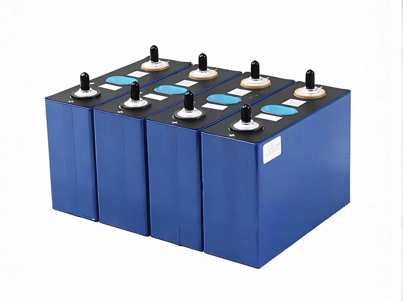
In this study, I designed two liquid cooling plate configurations: one with longitudinal cooling plates (Design 1) and one with transverse cooling plates (Design 2). The module consists of 18 prismatic lithium‑iron‑phosphate energy storage cells arranged in a 3‑series 6‑parallel configuration. Each cell has a nominal capacity of 20 Ah and dimensions of 148 mm × 26 mm × 92 mm. The cooling medium is water, and the plates are made of aluminum. Using COMSOL Multiphysics, I developed a three‑dimensional thermal‑fluidic model to evaluate the maximum temperature and maximum temperature difference of the module. I first validated the single‑cell thermal model by comparing simulation results with experimental data under a 0.5 C constant‑current constant‑voltage charging profile. The root‑mean‑square error was only 0.15 °C, confirming the accuracy of the model.
The heat generation rate of the energy storage cell is calculated using the Bernardi model:
$$
q = \frac{1}{V} \left[ (U_0 – U) – T \frac{dU_0}{dT} \right]
$$
where \( V \) is the cell volume, \( U_0 \) and \( U \) are the open‑circuit voltage and terminal voltage respectively, \( T \) is the temperature, and \( \frac{dU_0}{dT} \) is the temperature coefficient. The transient heat conduction equation in the anisotropic battery material is:
$$
\rho_k C_{p,k} \frac{\partial T}{\partial t} = \nabla \cdot (\lambda_k \nabla T) + q
$$
For the coolant flow inside the microchannels, the governing equations are:
$$
\rho_w (\mathbf{u}_w \cdot \nabla) \mathbf{u}_w = -\nabla p + \mu_w \nabla^2 \mathbf{u}_w
$$
$$
\nabla \cdot \mathbf{u}_w = 0
$$
$$
\rho_w c_w \left( \frac{\partial T}{\partial t} + \mathbf{u}_w \cdot \nabla T \right) = \nabla \cdot (k_w \nabla T)
$$
Convective heat transfer at the channel wall is described by:
$$
-\lambda \left( \frac{\partial T}{\partial n} \right)_w = h (T_w – T_f)
$$
I performed grid independence tests using three mesh densities (fine, normal, coarse) for both the single cell and the two module designs. The fine mesh was chosen for all subsequent simulations as it provided a good balance between accuracy and computational cost.
Thermal Performance Comparison of Two Liquid Cooling Designs
I first compared the cooling performance of Design 1 and Design 2 under 1 C and 3 C constant‑current charging. The initial temperature of the energy storage cells and the coolant was 25 °C, the coolant flow rate was 1 cm³/s, and each plate had 7 channels. The results are summarized in Table 1.
| Condition | Design | Max temperature (°C) | Max temperature difference (°C) |
|---|---|---|---|
| 1 C CC | Design 1 | 34.93 | 2.44 |
| Design 2 | 37.91 | 4.10 | |
| 3 C CC | Design 1 | 52.58 | 5.01 |
| Design 2 | 58.82 | 8.54 |
Under both low and high rates, Design 1 significantly outperformed Design 2 in reducing the maximum temperature and improving temperature uniformity. The reason is that the thermal conductivity of the energy storage cell in the Y‑direction (through the thickness) is much lower than in the X‑ and Z‑directions. In Design 2, the cooling plates are placed transversely, which limits heat transfer from the cells to the coolant. Therefore, all subsequent optimization studies are conducted using Design 1.
Parameter Optimization Under Constant‑Current Conditions
To systematically improve the liquid cooling system, I investigated the influence of four key parameters: coolant flow rate, coolant inlet temperature, number of cooling channels per plate, and inlet/outlet arrangement. The objectives are to minimize both the maximum temperature and the maximum temperature difference across the module of energy storage cells.
Effect of Coolant Flow Rate
I evaluated flow rates of 1, 2, and 3 cm³/s under 1 C, 2 C, and 3 C charging. As shown in Table 2, increasing the flow rate from 1 to 2 cm³/s reduced the maximum temperature by about 5 % under all rates, while a further increase to 3 cm³/s gave only marginal improvement (less than 2 %). The temperature difference increased slightly at higher flow rates due to the larger temperature gradient between inlet and outlet. Considering the pump energy consumption, a flow rate of 2 cm³/s is the optimal choice.
| Charging rate | Flow rate (cm³/s) | Max temperature (°C) | Max ΔT (°C) |
|---|---|---|---|
| 1 C | 1 | 33.05 | 2.31 |
| 2 | 31.27 | 2.38 | |
| 3 | 31.00 | 2.40 | |
| 2 C | 1 | 42.79 | 3.51 |
| 2 | 40.86 | 3.60 | |
| 3 | 40.30 | 3.62 | |
| 3 C | 1 | 49.66 | 4.41 |
| 2 | 46.90 | 4.56 | |
| 3 | 46.09 | 4.58 |
Effect of Coolant Inlet Temperature
I set the coolant inlet temperature to 20, 25, and 30 °C while keeping the cell initial temperature at 25 °C. Table 3 shows that reducing the coolant temperature by 5 °C decreases the module maximum temperature by approximately 3.5 °C, independent of the charging rate. However, the impact on temperature uniformity is modest: a 10 °C reduction in coolant temperature reduces the maximum temperature difference by only 0.5–1.2 °C. Given the additional cooling power required, 20 °C is recommended as the inlet temperature.
| Charging rate | Coolant temperature (°C) | Max temperature (°C) | Max ΔT (°C) |
|---|---|---|---|
| 1 C | 20 | 29.58 | 2.22 |
| 25 | 33.05 | 2.38 | |
| 30 | 36.49 | 2.85 | |
| 2 C | 20 | 39.28 | 3.60 |
| 25 | 42.79 | 3.71 | |
| 30 | 46.39 | 4.13 | |
| 3 C | 20 | 46.11 | 4.56 |
| 25 | 49.66 | 4.78 | |
| 30 | 53.34 | 5.33 |
Effect of Number of Cooling Channels
I varied the number of channels per plate from 5 to 7 to 9, while keeping the total cross‑sectional area per channel constant (5 mm × 5 mm). As listed in Table 4, increasing from 5 to 7 channels reduced the maximum temperature by about 9–11 %, but further increasing to 9 channels yielded only 3 % improvement. The maximum temperature difference increased slightly with more channels, likely because of more uneven flow distribution. Hence, 7 channels per plate offer the best trade‑off.
| Charging rate | Number of channels | Max temperature (°C) | Max ΔT (°C) |
|---|---|---|---|
| 1 C | 5 | 32.60 | 2.19 |
| 7 | 29.58 | 2.22 | |
| 9 | 28.69 | 2.25 | |
| 2 C | 5 | 43.84 | 3.52 |
| 7 | 39.28 | 3.60 | |
| 9 | 37.95 | 3.65 | |
| 3 C | 5 | 51.79 | 4.48 |
| 7 | 46.11 | 4.56 | |
| 9 | 44.55 | 4.63 |
Effect of Inlet/Outlet Arrangement
In the baseline design, all inlets were on the same side, leading to a temperature rise of the coolant along the flow direction. To mitigate this, I tested an alternating inlet arrangement where the inlets of adjacent channels are placed on opposite sides (see Table 5). This change had negligible effect on the maximum temperature but reduced the maximum temperature difference by 0.09 °C at 1 C and 0.42 °C at 3 C. The improvement is more pronounced at high rates where the coolant temperature gradient is larger.
| Charging rate | Inlet arrangement | Max temperature (°C) | Max ΔT (°C) |
|---|---|---|---|
| 1 C | Same side | 29.58 | 2.22 |
| Alternating | 29.48 | 2.13 | |
| 2 C | Same side | 39.28 | 3.60 |
| Alternating | 39.15 | 3.31 | |
| 3 C | Same side | 46.11 | 4.56 |
| Alternating | 45.93 | 4.14 |
Based on the above parametric studies, the optimal combination for the liquid cooling system under constant‑current conditions is: coolant flow rate of 2 cm³/s, coolant inlet temperature of 20 °C, 7 channels per plate, and alternating inlet arrangement. With this configuration, the module of energy storage cells achieves a maximum temperature of 29.58 °C at 1 C, 39.28 °C at 2 C, and 46.11 °C at 3 C, with corresponding temperature differences of 2.22, 3.60, and 4.56 °C.
Performance Under Realistic Peak‑Shaving and Frequency‑Regulation Conditions
To validate the liquid cooling system under practical operating profiles, I used typical current patterns from a real energy storage station for peak shaving and frequency regulation. The frequency‑regulation profile involves rapid charge‑discharge switching every 60 s, while the peak‑shaving profile consists of sustained charging or discharging periods interspersed with frequent transitions. I compared the performance of the optimal liquid cooling system with natural convection (no cooling) under these two scenarios.
Frequency‑Regulation Condition
Table 6 summarizes the module performance. The liquid cooling system reduced the maximum temperature from 49.14 °C (natural convection) to 43.86 °C, a drop of 10.74 %. The maximum temperature difference decreased from 6.33 °C to 3.54 °C, a 44.1 % improvement.
| Cooling method | Max temperature (°C) | Max ΔT (°C) |
|---|---|---|
| Natural convection | 49.14 | 6.33 |
| Optimal liquid cooling | 43.86 | 3.54 |
Peak‑Shaving Condition
Under the peak‑shaving profile (Table 7), the liquid cooling system kept the maximum temperature at 42.11 °C compared to 47.24 °C with natural convection, a reduction of 10.86 %. The maximum temperature difference dropped from 5.10 °C to 3.19 °C, a 37.45 % improvement.
| Cooling method | Max temperature (°C) | Max ΔT (°C) |
|---|---|---|
| Natural convection | 47.24 | 5.10 |
| Optimal liquid cooling | 42.11 | 3.19 |
These results confirm that the optimized liquid cooling system effectively controls both the peak temperature and the temperature uniformity of energy storage cells under dynamic real‑world conditions.
Variable Flow Rate Strategy for Improved Efficiency
In practical operation, the charge‑discharge rate of energy storage cells varies significantly over time. Using a constant coolant flow rate wastes energy during low‑load periods and may be insufficient during high‑load peaks. I therefore proposed a variable flow rate strategy: the coolant flow rate is reduced to 0.5 cm³/s during low‑rate periods and increased to 2.5 cm³/s during high‑rate periods, with a baseline of 2 cm³/s. The threshold is based on the instantaneous C‑rate of the cell.
Under the peak‑shaving profile, the variable flow rate strategy was compared with the constant flow rate of 2 cm³/s. As shown in Table 8, the maximum temperature of the module decreased from 42.11 °C to 39.84 °C (5.39 % lower), while the maximum temperature difference remained nearly identical (3.19 °C vs. 3.27 °C). Importantly, the total coolant volume consumed was reduced by 10.3 % (from 49 846 cm³ to 44 708 cm³). The variable flow approach not only improves cooling performance during high‑load events but also reduces pumping energy, making the system more efficient.
| Strategy | Max temperature (°C) | Max ΔT (°C) | Coolant volume (cm³) |
|---|---|---|---|
| Constant (2 cm³/s) | 42.11 | 3.19 | 49 846 |
| Variable (0.5/2.5 cm³/s) | 39.84 | 3.27 | 44 708 |
Conclusions
In this work, I systematically optimized a liquid cooling system for a module of lithium‑iron‑phosphate energy storage cells. The following conclusions can be drawn:
- The longitudinal cooling plate configuration (Design 1) significantly outperforms the transverse configuration (Design 2) in terms of both maximum temperature and temperature uniformity, because the cell’s thermal conductivity is anisotropic and higher in the longitudinal direction.
- Under constant‑current charging, the optimal parameter set is: coolant flow rate of 2 cm³/s, coolant inlet temperature of 20 °C, 7 channels per plate, and alternating inlet arrangement. This configuration keeps the module temperature well within the safe range even at 3 C.
- Under realistic peak‑shaving and frequency‑regulation profiles, the optimal liquid cooling system reduces the maximum temperature of energy storage cells by about 10.8 % and the maximum temperature difference by 37–44 % compared to natural convection.
- The variable flow rate strategy, which adjusts the coolant flow according to the instantaneous C‑rate, further lowers the peak temperature by 5.39 % while reducing coolant consumption by 10.3 %, thereby enhancing both thermal performance and energy efficiency.
These findings provide a practical guideline for designing efficient liquid cooling systems for large‑scale energy storage applications where energy storage cells are subjected to highly variable loads.