
The increasing integration of solar photovoltaic (PV) power generation into modern electrical grids presents both opportunities and challenges for system operators. Unlike conventional power sources, the output of a solar PV system is inherently intermittent and stochastic, primarily dependent on meteorological conditions such as solar irradiance and ambient temperature. This variability can lead to significant fluctuations in the net load (system load minus PV generation) seen by the grid, complicating tasks like unit commitment, economic dispatch, and ensuring grid stability. Therefore, accurate forecasting of the power output from solar PV systems—and by extension, the net system load—is paramount for the efficient, reliable, and cost-effective operation of power networks with high renewable penetration. This article presents a comprehensive methodology for load forecasting in solar PV-integrated power systems, focusing on a robust machine learning approach centered on the Extreme Learning Machine (ELM).
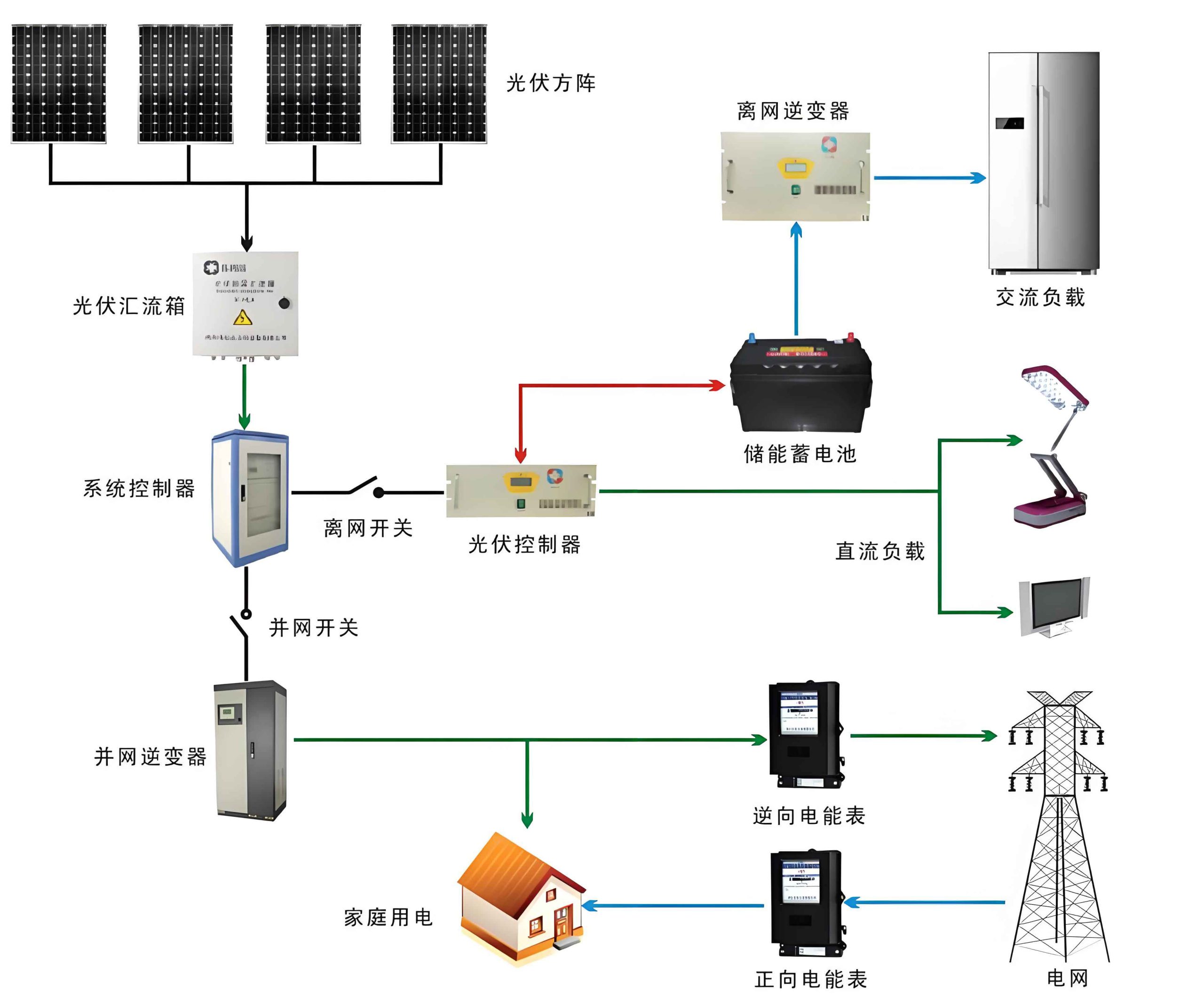
The core of the forecasting problem for a solar-augmented grid lies in modeling two interrelated components: the native system demand and the generated power from the PV installation. The total system load $L_{total}(t)$ at time $t$ is a complex function of historical load patterns, time-based variables (hour, day of week, season), and weather-sensitive components. The PV system’s output power $P_{pv}(t)$, however, is a direct function of the prevailing environmental conditions and the system’s physical characteristics. The net load $L_{net}(t)$ that must be supplied by conventional generators and other dispatchable resources is then given by:
$$L_{net}(t) = L_{total}(t) – P_{pv}(t)$$
Accurate forecasting requires reliable models for both $L_{total}(t)$ and $P_{pv}(t)$. We begin by establishing a foundational model for the photovoltaic component of the solar system.
1. Modeling the Solar Photovoltaic System Output
The electrical output of a PV cell, and by extension an array or a full-scale solar system, is fundamentally governed by the photovoltaic effect. A widely adopted model for a PV cell is the single-diode equivalent circuit model. The current-voltage (I-V) characteristic of this model is described by the following implicit equation:
$$I = I_{ph} – I_0 \left[ \exp\left(\frac{q(V + I R_s)}{n k T}\right) – 1 \right] – \frac{V + I R_s}{R_{sh}}$$
Where:
$I$: Output current of the PV cell.
$V$: Output voltage of the PV cell.
$I_{ph}$: Photogenerated current, which is directly proportional to the incident solar irradiance $G$: $I_{ph} \propto G$.
$I_0$: Reverse saturation current of the diode.
$q$: Electron charge ($1.602 \times 10^{-19}$ C).
$R_s$: Series resistance.
$R_{sh}$: Shunt resistance.
$n$: Diode ideality factor.
$k$: Boltzmann constant ($1.381 \times 10^{-23}$ J/K).
$T$: Cell temperature in Kelvin.
The maximum power point (MPP) power $P_{mpp}$ of a module is obtained by finding $V$ and $I$ such that $P = V \cdot I$ is maximized. For a solar system comprising $N_s$ modules in series and $N_p$ strings in parallel, the total DC power $P_{dc}$ is scaled accordingly. After accounting for inverter efficiency $\eta_{inv}$, the final AC output power $P_{pv}$ fed into the grid is:
$$P_{pv} = \eta_{inv} \cdot (N_s \cdot V_{mpp}) \cdot (N_p \cdot I_{mpp})$$
The primary stochastic input driving this model is the solar irradiance $G(t)$. Its variability is a major source of uncertainty in forecasting the output of any solar system. To incorporate this uncertainty into a probabilistic forecasting framework, the probability distribution of irradiance can be effectively modeled. For a given time period (e.g., an hour), the clear-sky index $k_t$, defined as the ratio of measured global horizontal irradiance (GHI) to clear-sky GHI, often follows a Beta distribution. The probability density function (PDF) for the irradiance $G$ is:
$$f(G) = \frac{\Gamma(\alpha + \beta)}{\Gamma(\alpha) \Gamma(\beta)} \left( \frac{G}{G_{max}} \right)^{\alpha-1} \left( 1 – \frac{G}{G_{max}} \right)^{\beta-1}, \quad 0 \leq G \leq G_{max}$$
Here, $G_{max}$ is the maximum possible irradiance (typically clear-sky irradiance), and $\alpha > 0$, $\beta > 0$ are shape parameters that can be estimated from historical data for different sky conditions, times of day, and seasons. This model allows us to generate stochastic scenarios of irradiance input for the PV power model, facilitating probabilistic load forecasts.
2. Theoretical Foundation for Load Forecasting
Forecasting, in a machine learning context, is the task of learning a functional mapping $F$ from a set of input features $\mathbf{x} \in \mathbb{R}^d$ to a target output $y \in \mathbb{R}$, based on a historical dataset $\mathcal{D} = \{(\mathbf{x}_i, y_i)\}_{i=1}^{N}$. For solar system net load forecasting, the input vector $\mathbf{x}_t$ at time $t$ is highly multidimensional and can include:
- Temporal Features: Hour-of-day, day-of-week, month, holiday flag.
- Historical Load & PV Data: Lagged values of $L_{net}$, $L_{total}$, and $P_{pv}$ (e.g., from the same hour on previous days, the immediate past hours).
- Meteorological Features: Forecasted and/or historical solar irradiance $G(t)$, temperature $T(t)$, humidity, cloud cover, wind speed.
- Solar System State: Module temperature, inverter status (if available).
The target output $y_t$ is typically the net load $L_{net}(t)$ for a future time horizon (e.g., the next hour, the next 24 hours). The goal is to find the function $F(\mathbf{x}; \boldsymbol{\theta})$, parameterized by $\boldsymbol{\theta}$, that minimizes the expected prediction error or risk $R(\boldsymbol{\theta})$ over the joint distribution of inputs and outputs $P(\mathbf{x}, y)$:
$$R(\boldsymbol{\theta}) = \mathbb{E}_{(\mathbf{x}, y) \sim P} \left[ \mathcal{L}(y, F(\mathbf{x}; \boldsymbol{\theta})) \right]$$
where $\mathcal{L}(\cdot)$ is a loss function, such as Mean Squared Error (MSE): $\mathcal{L}(y, \hat{y}) = (y – \hat{y})^2$. Since the true distribution $P$ is unknown, we minimize the empirical risk on the training data:
$$\hat{R}(\boldsymbol{\theta}) = \frac{1}{N} \sum_{i=1}^{N} \mathcal{L}(y_i, F(\mathbf{x}_i; \boldsymbol{\theta}))$$
The choice of the functional model $F$ and the optimization algorithm to find $\boldsymbol{\theta}$ is critical. This is where the Extreme Learning Machine offers distinct advantages for forecasting the complex, nonlinear behavior of a grid-integrated solar system.
3. Extreme Learning Machine (ELM) for Forecasting
The Extreme Learning Machine is a specialized type of single-hidden-layer feedforward neural network (SLFN) known for its extremely fast training speed and good generalization performance. The key innovation of ELM is the random initialization and fixing of the weights connecting the input layer to the hidden layer, followed by an analytical determination of the output layer weights via least-squares solution.
For a dataset with $N$ samples, input dimension $d$, and a hidden layer with $L$ neurons, the ELM model operates as follows:
- Random Feature Mapping: The input $\mathbf{x}_i$ is projected onto a random feature space. The hidden layer output for the $i$-th sample is a vector $\mathbf{h}_i \in \mathbb{R}^{L}$:
$$\mathbf{h}_i = g(\mathbf{W}_{in} \mathbf{x}_i + \mathbf{b})$$
where $\mathbf{W}_{in} \in \mathbb{R}^{L \times d}$ is a randomly assigned input weight matrix, $\mathbf{b} \in \mathbb{R}^{L}$ is a randomly assigned bias vector, and $g(\cdot)$ is a nonlinear activation function (e.g., sigmoid, ReLU, sine). - Linear Output Layer: The final prediction $\hat{y}_i$ is a linear combination of these random features:
$$\hat{y}_i = \mathbf{h}_i^T \boldsymbol{\beta}$$
where $\boldsymbol{\beta} \in \mathbb{R}^{L}$ is the output weight vector to be learned.
Collecting all $N$ samples, we can write the hidden layer output matrix $\mathbf{H}$ and the target vector $\mathbf{Y}$:
$$
\mathbf{H} = \begin{bmatrix}
\mathbf{h}_1^T \\
\mathbf{h}_2^T \\
\vdots \\
\mathbf{h}_N^T
\end{bmatrix} =
\begin{bmatrix}
g(\mathbf{w}_1 \cdot \mathbf{x}_1 + b_1) & \cdots & g(\mathbf{w}_L \cdot \mathbf{x}_1 + b_L)\\
\vdots & \ddots & \vdots\\
g(\mathbf{w}_1 \cdot \mathbf{x}_N + b_1) & \cdots & g(\mathbf{w}_L \cdot \mathbf{x}_N + b_L)
\end{bmatrix}, \quad
\mathbf{Y} = \begin{bmatrix}
y_1 \\
y_2 \\
\vdots \\
y_N
\end{bmatrix}
$$
The learning problem reduces to finding $\boldsymbol{\beta}$ that minimizes $||\mathbf{H}\boldsymbol{\beta} – \mathbf{Y}||^2$. The optimal solution, in the least-squares sense, is given by the Moore-Penrose generalized inverse (pseudoinverse) of $\mathbf{H}$:
$$\hat{\boldsymbol{\beta}} = \mathbf{H}^{\dagger} \mathbf{Y}$$
Where $\mathbf{H}^{\dagger} = (\mathbf{H}^T \mathbf{H})^{-1} \mathbf{H}^T$ if $\mathbf{H}^T \mathbf{H}$ is nonsingular. This one-step analytical solution bypasses the need for iterative gradient-based backpropagation, making ELM training orders of magnitude faster than conventional neural networks. This speed is a significant advantage when dealing with large volumes of historical data from the power grid and connected solar systems, and when frequent model retraining is required.
4. Integrated Forecasting Framework for Solar PV Systems
We propose an integrated forecasting framework that leverages the ELM’s strengths to predict the net load $L_{net}$. Two primary architectural approaches can be considered:
Approach A: Direct Net Load Forecasting with a Single ELM
A single ELM model is trained to directly map the comprehensive input feature vector $\mathbf{x}_t$ (containing temporal, historical load/PV, and weather forecast data) to the target net load $L_{net}(t+k)$ for a future time step $t+k$. This is an end-to-end approach where the model implicitly learns the correlations and interactions between total load and PV generation.
Approach B: Two-Stage Forecasting with Separate ELM Models
This approach involves training two specialized ELM models:
- PV Power Forecaster (ELM-PV): Predicts $P_{pv}(t+k)$ based on features like forecasted irradiance $G(t+k)$, temperature $T(t+k)$, historical PV output, and solar system parameters.
- System Load Forecaster (ELM-Load): Predicts the total system load $L_{total}(t+k)$ based on temporal features, historical load data, and non-solar weather variables (e.g., temperature for heating/cooling demand).
The final net load forecast is then obtained by subtraction:
$$\hat{L}_{net}(t+k) = \hat{L}_{total}(t+k) – \hat{P}_{pv}(t+k)$$
This modular approach offers transparency and allows for independent validation and improvement of each component model.
The table below summarizes the key features and inputs for these two approaches:
| Forecasting Approach | Model(s) Used | Primary Input Features | Target Output |
|---|---|---|---|
| Direct Net Load Forecast | Single ELM | Time vars, Lagged($L_{net}$, $L_{total}$, $P_{pv}$), Forecast(G, T, …) | $L_{net}(t+k)$ |
| Two-Stage Forecast | ELM-Load & ELM-PV | ELM-Load: Time vars, Lagged($L_{total}$), T, … ELM-PV: Forecast(G, T), Lagged($P_{pv}$), system params |
$L_{total}(t+k)$ & $P_{pv}(t+k)$ |
5. Data Preprocessing and Feature Engineering
The performance of any ELM-based forecast for a solar system is heavily dependent on the quality and relevance of the input data. Essential preprocessing steps include:
- Normalization/Standardization: Input features should be scaled to a common range (e.g., [0,1]) or distribution (zero mean, unit variance) to ensure stable and efficient learning. For a feature $x$:
$$x’ = \frac{x – \min(x)}{\max(x) – \min(x)} \quad \text{or} \quad x’ = \frac{x – \mu_x}{\sigma_x}$$ - Handling Missing Data: Gaps in irradiance, load, or temperature records must be addressed via interpolation, imputation, or deletion.
- Feature Engineering: Creating derived features can significantly improve forecasts. Examples include:
- Cyclical encoding of hour and month using sine/cosine transformations: $hour\_sin = \sin(2\pi * hour / 24)$, $hour\_cos = \cos(2\pi * hour / 24)$.
- Statistical features over rolling windows: mean and standard deviation of load and irradiance over the past 3, 6, or 24 hours.
- Interaction terms between key variables, such as $(G \times T)$.
- Training/Validation/Test Split: Temporal splitting must be used to avoid data leakage. For instance, use data from years 1-2 for training, year 3 for validation (hyperparameter tuning), and year 4 for final testing.
6. Experimental Analysis and Performance Metrics
To evaluate the proposed ELM-based methodology, a case study was conducted using historical data from a power grid region with significant solar PV penetration. The dataset included hourly records of system load, measured PV plant output, and local meteorological data (irradiance, temperature) over three years.
The Two-Stage Forecasting approach (Approach B) was implemented. The hyperparameters for both ELM models, such as the number of hidden neurons $L$ and the activation function $g(\cdot)$, were optimized using grid search on the validation set. The final models were compared against several benchmarks:
- Persistence Forecast: $\hat{L}_{net}(t+1) = L_{net}(t)$.
- Autoregressive Integrated Moving Average (ARIMA): A classic statistical time-series model.
- Standard Artificial Neural Network (ANN): Trained with backpropagation.
The following table summarizes the forecasting performance for a 24-hour ahead prediction horizon, measured on the independent test set. Key metrics include Mean Absolute Error (MAE), Root Mean Square Error (RMSE), and Mean Absolute Percentage Error (MAPE).
| Forecasting Model | MAE (MW) | RMSE (MW) | MAPE (%) |
|---|---|---|---|
| Proposed ELM-based Framework | 2.15 | 3.02 | 0.85 |
| Persistence Forecast | 8.47 | 10.89 | 3.92 |
| ARIMA | 5.33 | 7.21 | 2.15 |
| Standard ANN | 3.78 | 5.14 | 1.52 |
The results clearly demonstrate the superiority of the ELM-based approach. It achieved the lowest error across all metrics. The MAPE below 1% indicates a highly accurate forecast, which is operationally valuable for grid management. The ELM framework’s performance can be attributed to its ability to efficiently model the complex nonlinear relationships between the multitude of input factors—temporal patterns, weather dynamics, and the specific generation profile of the solar system—and the target net load.
7. Conclusion and Future Directions
Accurate load forecasting is a critical enabler for the secure and economic integration of variable renewable energy sources like solar photovoltaic power. This article has detailed a comprehensive methodology for forecasting the net load of a power system with significant PV generation, utilizing the power and efficiency of Extreme Learning Machines. By establishing a solid foundation in PV system modeling, articulating the forecasting problem within a machine learning risk minimization framework, and leveraging the unique fast-training characteristic of ELMs, the proposed approach delivers high-accuracy predictions.
The experimental validation confirms that the ELM-based framework can effectively capture the intricate dependencies in the data, outperforming traditional statistical and neural network benchmarks. The ability to maintain a mean absolute percentage error below 1% for net load forecasting underscores its practical utility for grid operators managing the balance between supply and demand in a modern, renewable-heavy solar system-integrated grid.
Future research directions could explore several enhancements: 1) Developing ensemble ELM models to further improve robustness and accuracy. 2) Incorporating probabilistic forecasting by using the ELM framework to predict prediction intervals or full density functions of the net load, which is crucial for risk-aware decision-making. 3) Implementing online sequential ELM (OS-ELM) for real-time, adaptive forecasting as new data from the solar system and grid streams in continuously. These advancements will further solidify the role of advanced machine learning techniques in building a resilient and smart power infrastructure.