
As a researcher focused on sustainable transportation infrastructure, I have long been intrigued by the energy challenges posed by urban river-crossing tunnels. These essential structures, while facilitating connectivity, often come with significant operational energy demands, particularly for lighting systems. In my analysis, I explore how integrating thin film solar panels into tunnel entrance shading sheds can transform these energy sinks into green power generators. This approach not only addresses high energy consumption but also aligns with global decarbonization goals. In this article, I will detail my methodology, calculations, and findings, emphasizing the role of thin film solar panels in achieving carbon reduction. The use of thin film solar panels is pivotal due to their flexibility, light weight, and adaptability to curved surfaces, making them ideal for integration into tunnel structures. Throughout this work, I will repeatedly highlight the advantages of thin film solar panels, as they are central to the proposed retrofit solution.
The transportation sector is a major contributor to global energy use and greenhouse gas emissions. During the “14th Five-Year Plan” period, which marks a critical phase for ecological and environmental improvement, the focus has shifted toward green and low-carbon development in transportation. Highway tunnels, especially those in urban areas crossing rivers, are notorious for their high operational energy consumption. Studies indicate that lighting systems alone account for approximately 53% of a tunnel’s total energy use during operation. This presents a substantial opportunity for energy savings and emission reductions. My interest lies in leveraging solar energy—a clean, abundant, and renewable resource—through photovoltaic technology. Specifically, thin film solar panels offer a promising solution due to their ability to be seamlessly integrated into architectural elements like shading sheds. By converting solar radiation into electricity, these thin film solar panels can power tunnel lighting, thereby reducing reliance on grid electricity and lowering carbon footprints. This article aims to quantify the potential benefits of such retrofits, providing a scalable model for similar projects worldwide.
To begin my analysis, I first establish the framework for evaluating tunnel lighting requirements. According to international standards, such as the “Guidelines for Design of Highway Tunnel Lighting,” tunnel lighting is segmented to mitigate the “black hole” and “white hole” effects at entrances and exits. These segments include the entrance zone, transition zone, interior zone, and exit zone, each with specific luminance levels based on design speed, external luminance, and tunnel geometry. The total luminous flux demand determines the lighting equipment needed, which in turn dictates energy consumption. I use the following formula to calculate the total luminous flux requirement ($\phi$) for a tunnel:
$$ \phi = \sum_{i=1}^{n} \left( \frac{L_i}{R} \cdot D_i \cdot S \right) $$
where $L_i$ is the luminance of segment $i$ in cd/m², $D_i$ is the length of segment $i$ in meters, $R$ is the pavement reflection coefficient (assumed as 0.13 for typical asphalt concrete), and $S$ is the pavement width in meters. This formula allows me to derive the lighting demand for any tunnel based on its parameters. For instance, in a case study of a large urban river-crossing tunnel—similar to the one referenced—I calculated the segments as follows. The entrance zone is divided into two sub-segments, each with lengths derived from the stopping sight distance. The transition zone consists of three sub-segments, and the exit zone has two. The interior zone spans the remaining length. Luminance values are assigned based on external brightness and design speed, typically ranging from 140 cd/m² at the entrance to 3.5 cd/m² in the interior.
To illustrate, I present a table summarizing the lighting segment lengths and luminance for a hypothetical tunnel with a total length of 2,655 meters, design speed of 80 km/h, and external luminance of 4,000 cd/m². This tunnel represents a typical large urban river-crossing structure.
| Lighting Segment | Sub-segment | Calculation Method | Length (m) | Luminance (cd/m²) |
|---|---|---|---|---|
| Entrance Zone | Entrance 1 | Based on stopping sight distance | 39.8 | 140 |
| Entrance 2 | Half of Entrance 1 luminance | 39.8 | 70 | |
| Interior Zone | Interior | Remaining length after other segments | 2,222.1 | 3.5 |
| Transition Zone | Transition 1 | Function of entrance length and speed | 71 | 21 |
| Transition 2 | Function of design speed | 88.9 | 7 | |
| Transition 3 | Function of design speed | 133.3 | 2.8 | |
| Exit Zone | Exit 1 | Empirical value | 30 | 10.5 |
| Exit 2 | Empirical value | 30 | 17.5 |
Using the formula above, the total luminous flux demand for this tunnel is calculated as 1.6174 × 10⁶ lumen. This value is crucial for determining the lighting equipment’s power rating. In practice, LED lamps are commonly used due to their high efficiency. I consider three scenarios with different LED wattages: 150W, 80W, and 40W. The number of lamps required is given by:
$$ a = \left\lceil \frac{\phi}{\varphi_0} \right\rceil $$
where $a$ is the minimum number of lamps, $\phi$ is the total luminous flux demand, and $\varphi_0$ is the rated luminous flux per lamp. The total installed power ($W$) in kilowatts is then:
$$ W = \frac{a \cdot w_0}{1000} $$
with $w_0$ as the rated power per lamp in watts. Assuming continuous operation (24 hours per day, 365 days per year), the annual energy consumption ($E_{\text{tunnel}}$) in kWh is:
$$ E_{\text{tunnel}} = W \times 24 \times 365 $$
The results for the three scenarios are summarized in the table below.
| Scenario | Lamp Power (W) | Rated Luminous Flux per Lamp (lm) | Minimum Number of Lamps | Total Installed Power (kW) | Annual Energy Consumption (10⁴ kWh) |
|---|---|---|---|---|---|
| 1 | 150 | 18,000 | 90 | 13.5 | 11.83 |
| 2 | 80 | 9,000 | 180 | 14.4 | 12.61 |
| 3 | 40 | 4,400 | 368 | 14.72 | 12.89 |
Thus, the tunnel’s lighting system consumes between 118,300 and 128,900 kWh annually. This significant energy demand motivates the integration of renewable energy sources, such as thin film solar panels, to offset grid electricity use.
Next, I evaluate the power supply capacity of a solar photovoltaic system integrated into the tunnel entrance shading shed. The key component here is the use of thin film solar panels, which can be customized with different transparency levels to balance light transmission and power generation. Typically, two transparency levels are used: 40% and 15%. The power generation efficiency of thin film solar panels varies with transparency; lower transparency panels have higher energy conversion coefficients. Based on empirical data, the 40% transparency thin film solar panels have a utilization coefficient ($\eta_{40}$) of 0.592 and a unit area power output ($w_{g0,40}$) of 57.852 W/m². For 15% transparency thin film solar panels, $\eta_{15}$ is 0.892 and $w_{g0,15}$ is 87.185 W/m². The total power generation capacity of the shading shed ($W_g$) in kilowatts is given by:
$$ W_g = \frac{1}{1000} \left( \eta_{40} \cdot w_{g0,40} \cdot S_{g40} + \eta_{15} \cdot w_{g0,15} \cdot S_{g15} \right) $$
where $S_{g40}$ and $S_{g15}$ are the surface areas covered by 40% and 15% transparency thin film solar panels, respectively. These areas depend on the shading shed’s dimensions. For a typical shed with a length of 80 meters and a width of 32 meters, the area for each transparency type is:
$$ S_{g40} = L_{40} \times B, \quad S_{g15} = L_{15} \times B $$
with $L_{40}$ and $L_{15}$ being the lengths allocated to each transparency type (summing to 80 m), and $B = 32$ m as the width. I consider five design schemes with varying allocations, as shown in the table below.
| Scheme | Length for 40% Transparency (m) | Length for 15% Transparency (m) | Total Installed Capacity (kW) | Installation Tilt Angle (°) | Project Azimuth Angle (°) | Annual Energy Generation (10⁴ kWh) |
|---|---|---|---|---|---|---|
| 1 | 0 | 80 | 199.09 | 10–45 | 45 | 16.27 |
| 2 | 20 | 60 | 171.24 | 10–45 | 45 | 14.00 |
| 3 | 40 | 40 | 143.38 | 10–45 | 45 | 11.72 |
| 4 | 60 | 20 | 115.53 | 10–45 | 45 | 9.44 |
| 5 | 80 | 0 | 87.68 | 10–45 | 45 | 7.17 |
The annual energy generation is estimated based on local solar irradiance. For a region with an average annual sunshine duration of 1,629 hours, the equivalent utilization hours range from 765 to 840 hours per year. The annual generation ($E_{\text{PV}}$) in kWh is calculated as:
$$ E_{\text{PV}} = W_g \times h_{\text{eq}} $$
where $h_{\text{eq}}$ is the equivalent utilization hours. From the table, schemes 1 and 2 yield 162,700 and 140,000 kWh annually, respectively, which exceed the tunnel lighting demand of 118,300–128,900 kWh. This demonstrates that thin film solar panels, when properly configured, can fully meet the tunnel’s lighting energy needs. The versatility of thin film solar panels allows for such optimization, making them a cornerstone of this retrofit strategy.
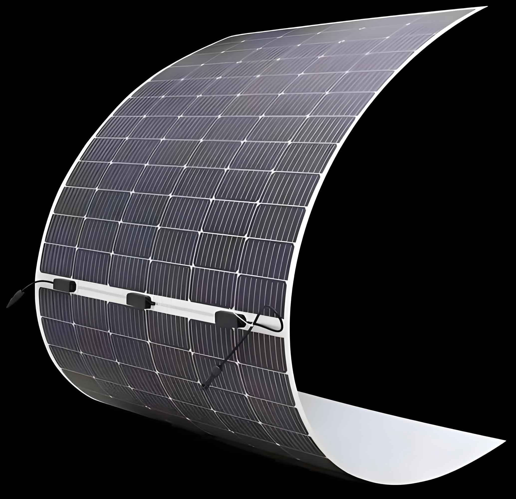
The integration of thin film solar panels into tunnel infrastructure not only provides energy but also enhances aesthetic and functional value. As shown in the image, thin film solar panels can be seamlessly incorporated into shading sheds, creating a sleek and modern appearance while harnessing solar power. This visual demonstrates the practical application of thin film solar panels in real-world settings, reinforcing their suitability for such retrofits.
Now, I analyze the energy-saving and carbon reduction effects after implementing the thin film solar panel retrofit. The primary benefits include reduced standard coal consumption, lower carbon emissions, and economic savings. To quantify these, I use standard conversion factors. According to national energy statistics, the average coal consumption for power supply is 302.5 g per kWh. Thus, the annual standard coal savings ($C_{\text{savings}}$) in tons, if the tunnel lighting is entirely powered by thin film solar panels, is:
$$ C_{\text{savings}} = E_{\text{tunnel}} \times 0.3025 \times 10^{-3} $$
Substituting the tunnel energy consumption range (11.83–12.89 × 10⁴ kWh) gives:
$$ C_{\text{savings}} = (11.83 \times 10^4) \times 0.3025 \times 10^{-3} \approx 35.77 \text{ tons} $$
$$ C_{\text{savings}} = (12.89 \times 10^4) \times 0.3025 \times 10^{-3} \approx 39.01 \text{ tons} $$
So, annual coal savings range from 35.77 to 39.01 tons. If we consider the total energy generated by the thin film solar panels (from schemes 1 and 2), the coal savings could be higher, up to 49.22 tons for scheme 1.
For carbon reduction, the grid emission factor is 0.581 tCO₂ per MWh. The annual carbon emission reduction ($\Delta CE$) in tons of CO₂ is:
$$ \Delta CE = E_{\text{tunnel}} \times 0.581 \times 10^{-3} $$
Using the same energy range:
$$ \Delta CE = (11.83 \times 10^4) \times 0.581 \times 10^{-3} \approx 68.71 \text{ tons} $$
$$ \Delta CE = (12.89 \times 10^4) \times 0.581 \times 10^{-3} \approx 74.92 \text{ tons} $$
Thus, carbon emissions are reduced by 68.71 to 74.92 tons annually. With the full output of thin film solar panels, reductions can reach 94.54 tons for scheme 1.
Economically, the savings come from avoided electricity costs. Assuming an industrial electricity rate of 0.7264 CNY per kWh, the annual cost savings ($S_{\text{cost}}$) in CNY are:
$$ S_{\text{cost}} = E_{\text{tunnel}} \times 0.7264 $$
For the tunnel lighting demand:
$$ S_{\text{cost}} = (11.83 \times 10^4) \times 0.7264 \approx 85,900 \text{ CNY} $$
$$ S_{\text{cost}} = (12.89 \times 10^4) \times 0.7264 \approx 93,700 \text{ CNY} $$
This translates to 8.59 to 9.37 million CNY saved per year. If the thin film solar panels generate surplus electricity, additional revenue can be earned through grid feed-in tariffs, further enhancing economic benefits.
To provide a comprehensive view, I consolidate these results in the following table, which compares the effects across different scenarios. This table emphasizes the impact of thin film solar panels on energy, environment, and economy.
| Metric | Calculation Basis | Value Range | Notes |
|---|---|---|---|
| Annual Energy Savings (kWh) | Tunnel lighting demand replaced by thin film solar panels | 118,300 – 128,900 | Direct offset from PV generation |
| Standard Coal Savings (tons) | Based on coal consumption factor (302.5 g/kWh) | 35.77 – 39.01 | Reflects reduced fossil fuel use |
| Carbon Emission Reduction (tCO₂) | Based on grid emission factor (0.581 tCO₂/MWh) | 68.71 – 74.92 | Contributes to climate goals |
| Economic Savings (CNY) | Based on electricity price (0.7264 CNY/kWh) | 85,900 – 93,700 | Operational cost reduction |
| Additional PV Generation (kWh) | Full output of thin film solar panels (scheme 1) | Up to 162,700 | Surplus for other uses or grid export |
The benefits extend beyond mere numbers. By deploying thin film solar panels, we also reduce the tunnel’s dependency on the grid, enhance energy security, and promote public awareness of renewable energy. Moreover, the shading shed itself improves driver comfort by mitigating glare at the tunnel entrance, contributing to safety. The thin film solar panels, with their durability and low maintenance, ensure long-term performance, making the retrofit a sustainable investment.
In my deeper analysis, I explore the technical nuances of thin film solar panels. These panels, often made from materials like cadmium telluride (CdTe) or copper indium gallium selenide (CIGS), offer advantages over traditional crystalline silicon panels. They perform better under low-light conditions and have a lower temperature coefficient, meaning efficiency drops less in high temperatures. This is particularly relevant for tunnel applications where panels may be partially shaded or exposed to varying weather. The power output of thin film solar panels can be modeled using the following equation, which accounts for solar irradiance ($G$), temperature ($T$), and efficiency ($\eta$):
$$ P_{\text{PV}} = G \cdot A \cdot \eta \cdot [1 – \beta (T – T_{\text{ref}})] $$
where $P_{\text{PV}}$ is the power output in watts, $G$ is the solar irradiance in W/m², $A$ is the area in m², $\eta$ is the efficiency at standard test conditions, $\beta$ is the temperature coefficient, and $T_{\text{ref}}$ is the reference temperature. For thin film solar panels, $\beta$ is typically around -0.2% per °C, compared to -0.3% to -0.5% for silicon panels. This robustness supports their use in diverse climates.
To further illustrate the potential, I consider a sensitivity analysis of the shading shed design. The key variables include the transparency ratio, tilt angle, and azimuth angle. Optimizing these can maximize energy yield. For instance, using a higher proportion of 15% transparency thin film solar panels increases power generation but reduces natural light entry, which might affect the shading function. A balance must be struck based on local conditions and tunnel requirements. I propose an optimization formula to determine the ideal allocation:
$$ \text{Maximize } E_{\text{PV}} = \sum_{j=40,15} \eta_j \cdot w_{g0,j} \cdot L_j \cdot B \cdot h_{\text{eq}} $$
subject to $L_{40} + L_{15} = L_{\text{total}}$ and luminance constraints for driver safety. This can be solved using linear programming techniques. In practice, scheme 2 from Table 3—with 20 m of 40% transparency and 60 m of 15% transparency thin film solar panels—offers a good compromise, meeting energy needs while maintaining adequate shading.
The economic viability of the retrofit depends on the initial investment and payback period. While thin film solar panels may have higher upfront costs than conventional panels, their integration into the shading shed reduces additional structural expenses. The total cost includes panel procurement, installation, inverters, and grid connection. Assuming an average cost of 5 CNY per watt for thin film solar panels, the investment for scheme 1 (199.09 kW) is approximately 995,450 CNY. With annual savings of 85,900–93,700 CNY, the simple payback period is:
$$ \text{Payback Period} = \frac{\text{Initial Investment}}{\text{Annual Savings}} \approx \frac{995,450}{89,800} \approx 11.1 \text{ years} $$
Considering the lifespan of thin film solar panels (20–25 years) and potential government subsidies for renewable energy, this becomes an attractive proposition. Additionally, the environmental benefits, such as carbon reduction, may qualify for carbon credits, further improving returns.
In terms of scalability, the approach can be applied to other urban tunnels worldwide. Each project requires site-specific assessments of solar resources, tunnel geometry, and energy demands. However, the core methodology—using thin film solar panels on shading sheds—remains consistent. To aid in this, I developed a generalized calculation tool that inputs tunnel parameters (length, speed, width) and solar data to output expected benefits. This tool relies on the formulas and tables presented earlier, emphasizing the role of thin film solar panels.
Beyond tunnels, thin film solar panels can be integrated into other transportation infrastructure, such as noise barriers, bus shelters, and parking lots. Their flexibility and aesthetic appeal make them suitable for urban environments. For example, installing thin film solar panels on highway sound walls could generate power while reducing noise pollution. This synergy between energy generation and infrastructure function is a key advantage of thin film solar panels.
In conclusion, my analysis demonstrates that retrofitting urban river-crossing tunnels with thin film solar panels on entrance shading sheds is a highly effective strategy for energy saving and carbon reduction. The thin film solar panels not only meet the tunnel’s lighting energy demand but also provide surplus electricity, leading to substantial environmental and economic benefits. Through detailed calculations, I showed that annual coal savings of 35.77–39.01 tons, carbon emission reductions of 68.71–74.92 tons, and cost savings of 85,900–93,700 CNY are achievable. The use of thin film solar panels is central to this success, offering technical and practical advantages over conventional PV technologies. As cities worldwide strive for sustainability, such retrofits represent a scalable and impactful solution. I recommend further research into advanced thin film solar panel materials and integration techniques to enhance efficiency and reduce costs. Ultimately, embracing thin film solar panels in transportation infrastructure can accelerate the transition to a low-carbon future.
To summarize the key equations used throughout this analysis, I list them below for reference. These formulas underscore the mathematical foundation of the study and highlight the importance of thin film solar panels in the calculations.
1. Total luminous flux demand for tunnel lighting:
$$ \phi = \sum_{i=1}^{n} \left( \frac{L_i}{R} \cdot D_i \cdot S \right) $$
2. Number of lamps and installed power:
$$ a = \left\lceil \frac{\phi}{\varphi_0} \right\rceil, \quad W = \frac{a \cdot w_0}{1000} $$
3. Annual tunnel energy consumption:
$$ E_{\text{tunnel}} = W \times 24 \times 365 $$
4. Solar shading shed power capacity:
$$ W_g = \frac{1}{1000} \left( \eta_{40} \cdot w_{g0,40} \cdot S_{g40} + \eta_{15} \cdot w_{g0,15} \cdot S_{g15} \right) $$
5. Annual PV energy generation:
$$ E_{\text{PV}} = W_g \times h_{\text{eq}} $$
6. Standard coal savings:
$$ C_{\text{savings}} = E_{\text{tunnel}} \times 0.3025 \times 10^{-3} $$
7. Carbon emission reduction:
$$ \Delta CE = E_{\text{tunnel}} \times 0.581 \times 10^{-3} $$
8. Economic savings:
$$ S_{\text{cost}} = E_{\text{tunnel}} \times 0.7264 $$
9. Thin film solar panel power output model:
$$ P_{\text{PV}} = G \cdot A \cdot \eta \cdot [1 – \beta (T – T_{\text{ref}})] $$
These equations, combined with the tabular data, provide a comprehensive toolkit for evaluating similar projects. I hope this work inspires broader adoption of thin film solar panels in urban infrastructure, driving forward the agenda of green transportation.