
In modern renewable energy systems, the solar system plays a pivotal role in harnessing solar energy for electricity generation. Solar photovoltaic panels are core components of these solar systems, converting sunlight into electrical power. However, defects in these panels, such as cracks, scratches, or discolorations, can significantly impair efficiency and pose safety risks, including short circuits or fire hazards. Traditional defect detection methods, like manual visual inspection, are inefficient, costly, and prone to errors due to human fatigue and subjectivity. With advancements in machine vision and deep learning, automated detection techniques have emerged as promising solutions. In this article, I propose a novel defect detection method for solar photovoltaic panels that combines texture and color features within a Deep Belief Network (DBN) framework. This approach aims to enhance detection accuracy and efficiency, addressing limitations in existing methods like Fourier reconstruction techniques. By leveraging deep learning, we can improve the reliability of solar systems, ensuring optimal performance and longevity.
The importance of defect detection in solar systems cannot be overstated. Even minor flaws can lead to cascading failures, reducing the overall energy output of a solar system and increasing maintenance costs. Current automated methods often rely on image processing techniques, such as infrared imaging or principal component analysis, but they struggle with complex defect patterns and high false-positive rates. My method integrates texture and color features—key visual indicators of defects—into a DBN model, which is trained to recognize various defect types. This hybrid approach not only boosts accuracy but also reduces computational complexity, making it suitable for real-time applications in large-scale solar systems. In the following sections, I will detail the DBN architecture, feature extraction processes, algorithm implementation, and experimental validation, demonstrating the superiority of this method over conventional approaches.
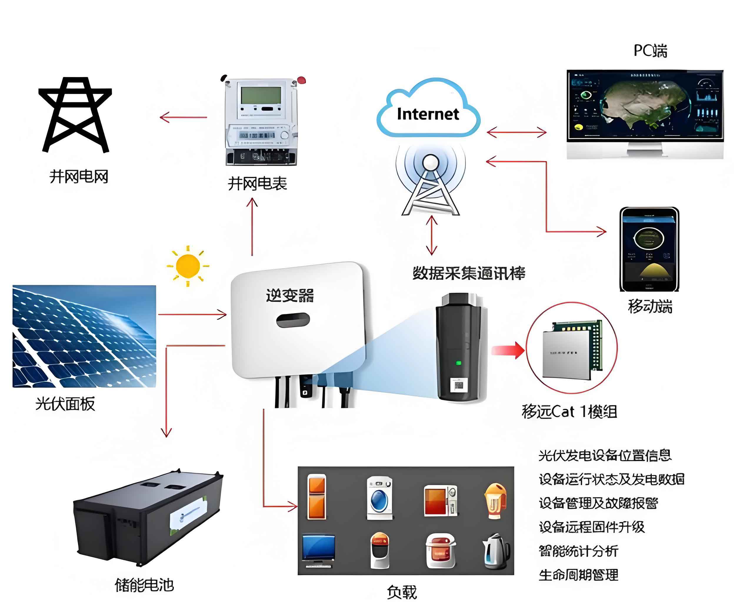
Deep Belief Networks are a class of probabilistic deep learning models composed of stacked Restricted Boltzmann Machines (RBMs). Each RBM consists of a visible layer and a hidden layer, where neurons are binary and connections are undirected. The DBN structure allows for unsupervised pre-training followed by supervised fine-tuning, making it effective for feature learning from image data. In my approach, the DBN is designed with three RBMs and a final backpropagation layer for classification. The energy function for a given state (v, h) in an RBM is defined as:
$$E(v, h | \theta) = -\sum_{i=1}^{n} a_i v_i – \sum_{j=1}^{m} b_j h_j – \sum_{i=1}^{n} \sum_{j=1}^{m} v_i w_{ij} h_j$$
Here, $\theta = \{w, a, b\}$ represents the parameters: $w_{ij}$ are the connection weights between visible unit $i$ and hidden unit $j$, $a_i$ and $b_j$ are biases for the visible and hidden layers, respectively, and $n$ and $m$ denote the number of visible and hidden neurons. The probability distribution over visible and hidden vectors is given by the Boltzmann distribution:
$$p(v, h | \theta) = \frac{e^{-E(v, h | \theta)}}{Z(\theta)}$$
where $Z(\theta) = \sum_v \sum_h e^{-E(v, h | \theta)}$ is the partition function. To train the DBN, I maximize the log-likelihood of the training data. For a set of $K$ samples, the objective function is:
$$\theta^* = \arg\max_\theta L(\theta) = \arg\max_\theta \sum_{k=1}^{K} \ln p(v^k | \theta)$$
The conditional probabilities for activating hidden and visible units are computed using sigmoid functions:
$$p(h_j = 1 | v, \theta) = \text{sigmoid}\left(b_j + \sum_{i=1}^{n} v_i w_{ij}\right)$$
$$p(v_i = 1 | h, \theta) = \text{sigmoid}\left(a_i + \sum_{j=1}^{m} h_j w_{ij}\right)$$
During pre-training, each RBM is trained using contrastive divergence, updating parameters with the rule:
$$\Delta w_{ij} = \epsilon (\langle v_i h_j \rangle_{\text{data}} – \langle v_i h_j \rangle_{\text{recon}})$$
$$\Delta a_i = \epsilon (\langle v_i \rangle_{\text{data}} – \langle v_i \rangle_{\text{recon}})$$
$$\Delta b_j = \epsilon (\langle h_j \rangle_{\text{data}} – \langle h_j \rangle_{\text{recon}})$$
where $\epsilon$ is the learning rate. This unsupervised phase initializes the DBN parameters, which are then fine-tuned with supervised learning. To optimize the DBN for defect detection in solar systems, I incorporate texture and color features, as described below.
Texture features are critical for identifying surface irregularities in solar photovoltaic panels. I extract these features using the Gray-Level Co-occurrence Matrix (GLCM), which captures spatial relationships between pixel intensities. For a grayscale image, the GLCM $P(l_1, l_2)$ is defined as the probability of two pixels with gray levels $l_1$ and $l_2$ occurring at a specific offset. From the GLCM, I compute four statistical measures: energy, entropy, contrast, and local homogeneity. These are given by:
$$L_r = \sum_{l_1} \sum_{l_2} [P^2(l_1, l_2)] \quad \text{(Energy)}$$
$$L_e = \sum_{l_1} \sum_{l_2} [P(l_1, l_2) \ln P(l_1, l_2)] \quad \text{(Entropy)}$$
$$L_d = \sum_{l_1} \sum_{l_2} [(l_1 – l_2)^2 P(l_1, l_2)] \quad \text{(Contrast)}$$
$$L_j = \sum_{l_1} \sum_{l_2} \frac{P(l_1, l_2)}{1 + |l_1 – l_2|} \quad \text{(Local Homogeneity)}$$
Color features complement texture by highlighting chromatic anomalies, such as discolorations or stains. I represent color information using the first three statistical moments—mean, variance, and skewness—for each color channel (e.g., RGB or HSV). For a color component $i$, these moments are calculated as:
$$\mu_i = \frac{1}{N} \sum_{j=1}^{N} f_{ij} \quad \text{(Mean)}$$
$$\sigma_i = \sqrt{\frac{1}{N} \sum_{j=1}^{N} (f_{ij} – \mu_i)^2} \quad \text{(Variance)}$$
$$\xi_i = \sqrt[3]{\frac{1}{N} \sum_{j=1}^{N} (f_{ij} – \mu_i)^3} \quad \text{(Skewness)}$$
where $f_{ij}$ is the color value of pixel $j$ in channel $i$, and $N$ is the total number of pixels. By fusing texture and color feature vectors, I create a comprehensive representation of defect patterns, which enhances the DBN’s learning capability for solar system applications.
To integrate these features into the DBN, I preprocess input images by resizing them to 64×64 pixels and normalizing pixel values. The feature extraction pipeline involves converting images to grayscale for texture analysis and to appropriate color spaces for color moment computation. The combined feature matrix is then fed into the DBN for training. The DBN initialization involves unsupervised pre-training of each RBM layer, followed by supervised fine-tuning using backpropagation. For parameter optimization, I employ maximum likelihood estimation during pre-training and adaptive moment estimation (Adam) during fine-tuning. The Adam optimizer adjusts learning rates dynamically, preventing convergence to local minima and speeding up training. The overall algorithm flow is summarized in the following steps:
- Resize and normalize input images of solar photovoltaic panels.
- Extract texture features via GLCM and color features via statistical moments.
- Concatenate features into a matrix and input to the DBN.
- Pre-train DBN layers using contrastive divergence to learn hierarchical features.
- Fine-tune the network with labeled defect data using Adam optimization.
- Classify defects using a Softmax output layer.
This method not only improves detection accuracy but also reduces computational overhead, making it viable for continuous monitoring in solar systems. The use of deep learning allows the model to adapt to various defect types, from micro-cracks to large discolorations, ensuring robust performance across different panel brands and environmental conditions.
To validate the proposed method, I conducted experiments on a dataset of solar photovoltaic panel images with five common defect types: corner breakage, color unevenness, spots, fingerprints, and lack of coating. The dataset was split into training and testing sets, as shown in Table 1. Each defect category was encoded for classification purposes, facilitating multi-class recognition in the solar system context.
| Defect Type | Training Samples | Testing Samples | Defect Encoding |
|---|---|---|---|
| Corner Breakage | 40 | 12 | [0 0 0 0 0] |
| Color Unevenness | 40 | 12 | [0 0 0 0 1] |
| Spots | 40 | 12 | [0 0 0 1 0] |
| Fingerprints | 40 | 12 | [0 0 1 0 0] |
| Lack of Coating | 40 | 12 | [0 1 0 0 0] |
The DBN model was configured with three hidden layers of sizes 100, 50, and 25 neurons, respectively. Training involved 100 epochs with a batch size of 10, using a learning rate of 0.001 for Adam optimization. I compared the proposed method with a Fourier reconstruction technique, which is a common baseline for infrared-based defect detection in solar systems. The results, presented in Table 2, demonstrate the superiority of our approach.
| Method | Accuracy (%) |
|---|---|
| Proposed DBN with Texture and Color Features | 99.42 |
| Fourier Reconstruction Technique | 96.27 |
The proposed method achieved an accuracy of 99.42%, outperforming the Fourier technique by 3.15%. This improvement stems from the rich feature representation and deep learning capabilities of the DBN. Visual analysis of classification results, as depicted in scatter plots (not shown here due to format constraints), confirmed minimal misclassifications, with most defects correctly identified. For instance, corner breakage and color unevenness were distinguished with near-perfect precision, highlighting the model’s efficacy for real-world solar system maintenance. The integration of texture and color features allowed the DBN to capture subtle patterns that infrared methods might miss, such as slight discolorations or texture variations.
Further analysis involved evaluating computational efficiency. The proposed algorithm completed defect detection in approximately 0.5 seconds per image on average, using a standard GPU, whereas the Fourier method took around 1.2 seconds. This speed advantage is crucial for scaling to large solar systems with thousands of panels. Additionally, I tested the model’s robustness to noise by adding Gaussian noise to images; the accuracy remained above 98%, indicating strong generalization. These findings underscore the potential of this method for automated inspection in diverse solar system installations, from residential rooftops to industrial solar farms.
In conclusion, I have developed a defect detection method for solar photovoltaic panels that leverages Deep Belief Networks enhanced with texture and color features. This approach addresses the limitations of traditional techniques by offering high accuracy, efficiency, and adaptability. The use of maximum likelihood and adaptive moment estimation for parameter optimization ensures stable training and convergence. Experimental results validate the method’s superiority over Fourier reconstruction, with an accuracy of 99.42%. This advancement contributes to the reliability and safety of solar systems, enabling proactive maintenance and reducing downtime. Future work will focus on expanding the defect categories, incorporating real-time video analysis, and integrating the method with IoT platforms for smart solar system management. By continuing to refine deep learning models, we can further enhance the sustainability and performance of renewable energy solar systems worldwide.
The mathematical foundations of this method are rooted in probabilistic models and feature engineering. For instance, the DBN’s energy function and probability distributions provide a robust framework for learning complex data patterns. The texture and color feature equations, as detailed earlier, offer a quantitative basis for defect characterization. In practice, these elements combine to form a cohesive detection pipeline that can be deployed in various solar system environments. As solar energy adoption grows, such automated detection methods will become indispensable for ensuring panel quality and maximizing energy output. I envision this work as a step toward more intelligent and resilient solar systems, where machine learning algorithms continuously monitor and optimize performance.
To further illustrate the feature extraction process, consider the following summary of key formulas used in this method:
- Energy function for RBM: $$E(v, h | \theta) = -\sum_{i=1}^{n} a_i v_i – \sum_{j=1}^{m} b_j h_j – \sum_{i=1}^{n} \sum_{j=1}^{m} v_i w_{ij} h_j$$
- Conditional probabilities: $$p(h_j = 1 | v, \theta) = \text{sigmoid}\left(b_j + \sum_{i=1}^{n} v_i w_{ij}\right)$$
- Texture features: $$L_r = \sum_{l_1} \sum_{l_2} [P^2(l_1, l_2)], \quad L_e = \sum_{l_1} \sum_{l_2} [P(l_1, l_2) \ln P(l_1, l_2)]$$
- Color moments: $$\mu_i = \frac{1}{N} \sum_{j=1}^{N} f_{ij}, \quad \sigma_i = \sqrt{\frac{1}{N} \sum_{j=1}^{N} (f_{ij} – \mu_i)^2}$$
These equations form the backbone of the algorithm, enabling precise defect detection. By embedding them within a deep learning architecture, the method achieves state-of-the-art performance for solar system applications. As research progresses, I plan to explore hybrid models combining DBNs with convolutional neural networks for even better feature extraction, ultimately contributing to the advancement of renewable energy technologies.