
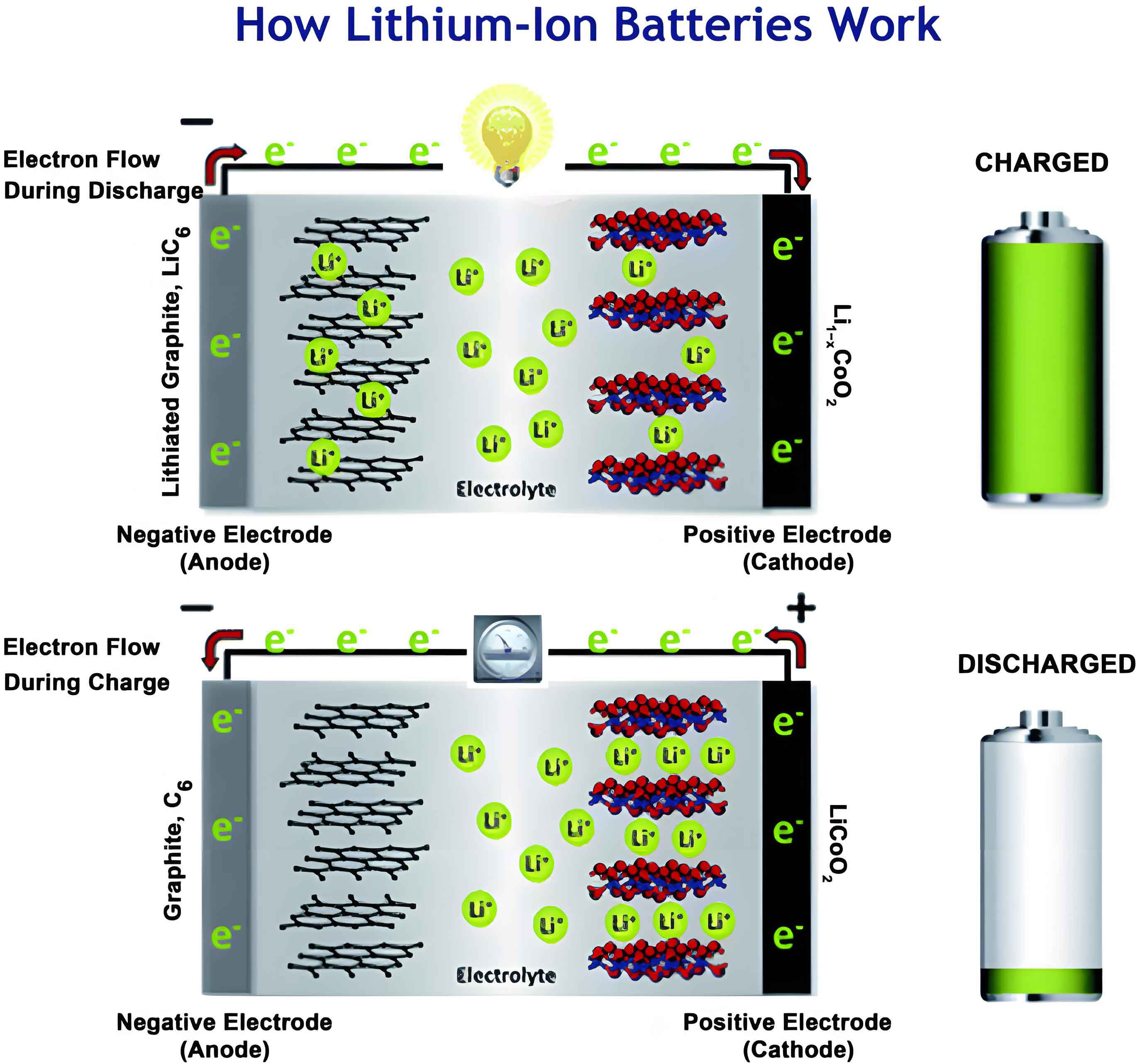
In recent years, lithium-ion batteries have become ubiquitous in modern technology, powering everything from portable electronics to electric vehicles and grid-scale energy storage systems. Their high energy density, long cycle life, and relatively low self-discharge rate make them a cornerstone of the renewable energy transition. However, as a lithium-ion battery undergoes repeated charge and discharge cycles, its performance gradually degrades due to complex electrochemical processes such as solid electrolyte interface growth, lithium plating, and active material loss. This degradation directly impacts the battery’s State of Health (SOH), a critical parameter defined as the ratio of its current maximum capacity to its initial nominal capacity. Accurate SOH estimation is paramount for ensuring safety, optimizing battery usage, preventing unexpected failures, and facilitating timely maintenance or replacement. My research focuses on overcoming the persistent challenges in data-driven SOH estimation, which include the selection of truly representative health indicators, the construction of models capable of capturing intricate feature relationships, and the optimization of these models for superior accuracy and robustness.
The journey toward reliable SOH estimation begins with data. In operational scenarios, discharge conditions can be highly dynamic and unpredictable, whereas charging protocols are often standardized and controlled. Therefore, I concentrate on extracting aging-related features from the charging phase of lithium-ion batteries. For a typical constant-current constant-voltage (CCCV) charge profile, several tell-tale signs of aging emerge: the constant-current (CC) charging duration shortens, the constant-voltage (CV) charging phase lengthens, and the incremental capacity (IC) curve—obtained by differentiating capacity with respect to voltage—shifts and diminishes. From these observations, I systematically extract eight key features: total charging time (F1), constant-current charging time (F2), constant-voltage charging time (F3), the integral area under the total charging current curve (F4), the area under the CC phase current curve (F5), the area under the CV phase current curve (F6), and the peak value (F7) along with its corresponding voltage (F8) from the IC curve. These features encapsulate the combined effects of internal resistance increase, loss of lithium inventory, and active material degradation within the lithium-ion battery.
Merely extracting features is insufficient; evaluating their quality and relevance is crucial. Traditional methods often rely on single metrics like the Pearson correlation coefficient (r) or Spearman’s rank coefficient (ρ) to gauge a feature’s relationship with SOH. While informative, such one-dimensional assessments can be misleading. A feature might have a high linear correlation but be highly sensitive to measurement noise, or it might exhibit a strong monotonic trend but lack a direct physical connection to the degradation mechanism. To address this, I propose a Comprehensive Feature Evaluation Index that appraises features from multiple, complementary perspectives: intrinsic relevance, cyclic stability, temporal dependency, entropy variability, and noise robustness.
The evaluation framework operates as follows. First, from a principle-based perspective, the Intrinsic Relevance (Int) is quantified using the Analytic Hierarchy Process (AHP), which assigns weights based on prior knowledge of each feature’s contribution to lithium-ion battery degradation. A consistent pairwise comparison matrix A is constructed, and its principal eigenvector provides the Int scores after passing consistency checks (CI, CR).
Second, from a statistical perspective, four indices are calculated:
1. Cyclic Stability (Cyc): Assessed using the Hurst exponent, indicating whether the feature’s evolution over cycles is smooth or erratic.
2. Temporal Dependency (Corr): Measured via the Spearman coefficient to evaluate monotonicity with cycle count.
$$ Corr = 1 – \frac{6\sum_{i=1}^{n} d_i^2}{n(n^2 – 1)} $$
where \(d_i\) is the rank difference for the i-th data point and \(n\) is the sample size.
3. Entropy Variability (Ent): Calculated using the sample skewness to measure the asymmetry in the feature’s distribution, which relates to the predictability of its degradation trend.
$$ Ent = \frac{n}{(n-1)(n-2)} \sum_{i=1}^{n} \left( \frac{x_i – \bar{x}}{s} \right)^3 $$
4. Noise Robustness (Rob): Calculated using the sample kurtosis to gauge the feature’s resistance to outliers and measurement noise.
$$ Rob = \frac{n(n+1)}{(n-1)(n-2)(n-3)} \sum_{i=1}^{n} \left( \frac{x_i – \bar{x}}{s} \right)^4 – \frac{3(n-1)^2}{(n-2)(n-3)} $$
In these formulas, \(x_i\) is the feature value, \(\bar{x}\) is the sample mean, and \(s\) is the sample standard deviation.
All scores for a given feature across the five indices (Int, Cyc, Corr, Ent, Rob) are normalized to a [0,1] range. A weighted sum is then computed, where the weight for each index is assigned based on the feature’s rank within that index, giving higher weight to better ranks. The final composite score \(Q_a\) for feature \(a\) is:
$$ Q_a = \sum_{b=1}^{5} w_{a,b} \cdot x^*_{a,b} $$
$$ w_{a,b} = \frac{9 – \text{rank}(x^*_{a,b}, b)}{9} $$
Here, \(x^*_{a,b}\) is the normalized score and \(\text{rank}(x^*_{a,b}, b)\) is its rank (1 to 8) among all features for index \(b\). This multi-faceted scoring system ensures that selected features are not only statistically correlated but also physically meaningful, stable over time, and resistant to disturbances. The following table exemplifies the normalized scores and final rankings for the eight extracted features from a sample dataset, clearly showing how the comprehensive evaluation can diverge from single-metric rankings.
| Feature | Int | Cyc | Corr | Ent | Rob | Composite Score (Q) | Rank |
|---|---|---|---|---|---|---|---|
| F1 | 0.15 | 0.84 | 0.99 | 0.10 | 0.50 | 2.07 | 4 |
| F2 | 0.14 | 0.84 | 0.98 | 0.09 | 0.51 | 2.24 | 3 |
| F3 | 0.05 | 0.83 | 0.89 | 0.15 | 0.60 | 1.98 | 5 |
| F4 | 0.17 | 0.80 | 0.99 | 0.13 | 0.62 | 2.68 | 1 |
| F5 | 0.16 | 0.80 | 0.99 | 0.14 | 0.50 | 2.25 | 2 |
| F6 | 0.10 | 0.74 | 0.97 | 0.11 | 0.47 | 1.60 | 6 |
| F7 | 0.07 | 0.61 | 0.98 | 0.10 | 0.43 | 1.05 | 7 |
| F8 | 0.05 | 0.72 | 0.75 | 0.16 | 0.15 | 0.27 | 8 |
With high-quality features selected, the next challenge is building a predictive model that can learn the complex, non-linear mapping from these features to the SOH of a lithium-ion battery. Simple models often fail to capture temporal dependencies and intricate patterns. Therefore, I design a hybrid neural network architecture that synergistically combines Convolutional Neural Networks (CNN), an Efficient Local Attention (ELA) mechanism, and a Bidirectional Gated Recurrent Unit (BiGRU). The CNN serves as a powerful spatial feature extractor, scanning the input feature vector for local patterns and hierarchies that might be indicative of specific degradation modes. However, not all extracted features or their interactions are equally important for predicting the SOH at a given cycle. This is where the Efficient Local Attention mechanism comes in. Integrated after the CNN layers, ELA allows the model to dynamically focus its “attention” on the most salient local features or feature combinations, weighting them more heavily in the subsequent processing stages. This mimics a form of automated feature re-evaluation within the model itself, enhancing its discriminative power. Finally, the refined feature sequence is fed into a BiGRU network. The BiGRU is exceptional at modeling sequential data because it processes information in both forward and backward directions. For a lithium-ion battery, the SOH at cycle \(t\) is inherently dependent not just on the current features but also on the historical degradation trajectory. The BiGRU captures these long-range temporal dependencies, remembering relevant past states and anticipating trends, which is crucial for accurate SOH estimation, especially during periods of non-linear capacity fade or regeneration. The state update equations for the BiGRU are as follows for the forward (\(\overrightarrow{h_t}\)) and backward (\(\overleftarrow{h_t}\)) passes:
Forward GRU:
$$ \begin{aligned}
z_t &= \sigma(W_{xz} x_t + W_{hz} \overrightarrow{h}_{t-1} + b_z) \\
r_t &= \sigma(W_{xr} x_t + W_{hr} \overrightarrow{h}_{t-1} + b_r) \\
\tilde{h}_t &= \tanh(W_{xh} x_t + r_t \odot (W_{hh} \overrightarrow{h}_{t-1}) + b_h) \\
\overrightarrow{h}_t &= z_t \odot \overrightarrow{h}_{t-1} + (1 – z_t) \odot \tilde{h}_t
\end{aligned} $$
Backward GRU (similar equations, processing sequence in reverse). The final hidden state \(h_t\) is a concatenation or linear combination of both directional states:
$$ h_t = V_t \overrightarrow{h}_t + v_t \overleftarrow{h}_t + k_t $$
While the CNN-ELA-BiGRU architecture is potent, its performance is highly sensitive to several hyperparameters: the learning rate, the number of hidden units in the BiGRU layers, and the regularization coefficient. Manually tuning these is tedious and often suboptimal. To fully automate and optimize the model, I employ the Golden Jackal Optimization (GJO) algorithm. GJO is a novel metaheuristic inspired by the cooperative hunting behavior of golden jackals. It is particularly effective because it maintains a balance between exploration (searching new areas of the hyperparameter space) and exploitation (refining good solutions), which helps avoid premature convergence to local optima—a common pitfall in optimization. The algorithm initializes a population of candidate solutions (hyperparameter sets). The position of each “jackal” is updated based on simulations of chasing and encircling prey (the optimal solution), guided by an energy factor \(E\) that decreases over iterations, and Levy flight random walks to enhance exploration. The core position update for a jackal is:
Prey searching (when \(|E| \geq 1\)):
$$ \begin{aligned}
Y_1(t) &= Y_M(t) – E \cdot |Y_M(t) – Z_L \cdot P(t)| \\
Y_2(t) &= Y_{FM}(t) – E \cdot |Y_{FM}(t) – Z_L \cdot P(t)|
\end{aligned} $$
Encircling prey (when \(|E| < 1\)):
$$ \begin{aligned}
Y_1(t) &= Y_M(t) – E \cdot |Z_L \cdot Y_M(t) – P(t)| \\
Y_2(t) &= Y_{FM}(t) – E \cdot |Z_L \cdot Y_{FM}(t) – P(t)|
\end{aligned} $$
$$ Y(t+1) = \frac{Y_1(t) + Y_2(t)}{2} $$
Here, \(Y_M\) and \(Y_{FM}\) represent the positions of the male and female jackal leading the hunt (the best solutions found), \(P(t)\) is the prey position (current best estimate), \(E\) is the escaping energy, and \(Z_L\) is a Levy flight-based random vector. GJO efficiently navigates the hyperparameter space to find the configuration that minimizes the prediction error on a validation set, thereby creating a finely-tuned GJO-CNN-ELA-BiGRU model for lithium-ion battery SOH estimation.
To rigorously validate the proposed method, I conducted extensive experiments on two widely recognized public datasets: NASA PCoE and CALCE. The NASA dataset comprises 18650-type lithium-ion batteries cycled under different ambient temperatures (4°C, 24°C, 43°C), while the CALCE dataset features CS2-type batteries. This variety is crucial for testing generalizability. The SOH is calculated as the ratio of discharge capacity in each cycle to the initial rated capacity. The experimental protocol involves using data from one or more batteries for training and evaluating the model on a different, unseen battery. To quantify performance, I use three standard error metrics: Root Mean Square Error (RMSE), Mean Absolute Error (MAE), and Mean Absolute Percentage Error (MAPE), defined as:
$$ \text{RMSE} = \sqrt{\frac{1}{N} \sum_{i=1}^{N} (y_i – \hat{y}_i)^2} $$
$$ \text{MAE} = \frac{1}{N} \sum_{i=1}^{N} |y_i – \hat{y}_i| $$
$$ \text{MAPE} = \frac{100\%}{N} \sum_{i=1}^{N} \left| \frac{y_i – \hat{y}_i}{y_i} \right| $$
where \(y_i\) is the true SOH, \(\hat{y}_i\) is the estimated SOH, and \(N\) is the number of cycles.
The first set of experiments demonstrates the superiority of the comprehensive feature evaluation index. I compared feature selection based on Pearson correlation (r), Spearman correlation (ρ), Principal Component Analysis (PCA), and my composite index. Using a simple CNN as the baseline predictor, the results consistently showed that features chosen by the composite index led to lower prediction errors across multiple battery pairs. For instance, when predicting battery B6 using B5 data, the composite index-selected features achieved an RMSE of 1.78%, outperforming the 2.40% from ρ-based selection and 2.42% from r-based selection. PCA, while reducing dimensionality, often discarded nuanced information, resulting in higher errors. This confirms that a multi-angle evaluation is essential for identifying the most robust and informative health indicators for a lithium-ion battery.
The second set of experiments pits the proposed GJO-CNN-ELA-BiGRU model against several state-of-the-art and baseline models, including standard LSTM, BiGRU, CNN-BiGRU, and the non-optimized CNN-ELA-BiGRU. All models were fed the same set of eight extracted features. The results, summarized in the table below, are compelling. The hybrid models consistently outperform the pure recurrent networks (LSTM, BiGRU), highlighting the benefit of CNN-based spatial feature extraction. Introducing the ELA mechanism into the CNN-BiGRU architecture provided a clear boost, reducing errors by enhancing focus on critical local patterns. Finally, the GJO-optimized version of the model achieved the best performance across almost all test scenarios. For example, in the challenging cross-temperature prediction from B5 (24°C) to B7 (24°C), the GJO-CNN-ELA-BiGRU model achieved an RMSE of 0.80% and a MAPE of 0.84%, significantly lower than the other contenders. This trend held even for batteries with less consistent aging patterns (like B18) or those cycled at different temperatures, proving the model’s robustness and strong generalization capability for lithium-ion battery SOH estimation.
| Training Set | Test Set | Model | MAPE (%) | RMSE (%) |
|---|---|---|---|---|
| B5 | B7 | LSTM | 1.17 | 0.95 |
| BiGRU | 1.12 | 0.92 | ||
| CNN-BiGRU | 1.08 | 0.97 | ||
| CNN-ELA-BiGRU | 1.00 | 0.89 | ||
| GJO-CNN-ELA-BiGRU | 0.84 | 0.80 | ||
| B5 | B18 | LSTM | 2.22 | 2.52 |
| CNN-ELA-BiGRU | 2.08 | 2.63 | ||
| GJO-CNN-ELA-BiGRU | 2.06 | 2.07 | ||
| B30 (43°C) | B31 (43°C) | GJO-CNN-ELA-BiGRU | 1.76 | 1.22 |
| B46 (4°C) | B48 (4°C) | GJO-CNN-ELA-BiGRU | 0.82 | 0.87 |
| CS35 | CS36 | GJO-CNN-ELA-BiGRU | 0.40 | 0.55 |
A third experiment was designed to evaluate the effectiveness of the GJO optimizer itself. I compared it against other popular metaheuristic algorithms—Particle Swarm Optimization (PSO), Grey Wolf Optimizer (GWO), and Sparrow Search Algorithm (SSA)—in tuning the hyperparameters of the CNN-ELA-BiGRU model. The objective was to minimize the MAE on a validation set. The GJO algorithm consistently found hyperparameter sets that yielded lower final prediction errors and did so with faster convergence. The table below shows a statistical summary over 30 independent runs for a specific test case (training on B18, testing on B7). GJO achieved the lowest mean error, the smallest variance (indicating high stability), and the quickest convergence time, solidifying its role as a superior optimizer for this application.
| Optimizer | Max Error (%) | Min Error (%) | Mean Error (%) | Variance (%) | Convergence Time (s) |
|---|---|---|---|---|---|
| PSO | 3.73 | 2.46 | 3.03 | 3.12 | 10.24 |
| GWO | 3.59 | 2.52 | 3.09 | 3.01 | 11.53 |
| SSA | 3.60 | 2.32 | 2.66 | 2.43 | 11.05 |
| GJO | 2.58 | 1.94 | 2.03 | 1.98 | 8.96 |
The results unequivocally demonstrate the efficacy of the proposed framework. The comprehensive feature evaluation index successfully identifies features that are not merely statistically correlated but are physically grounded, temporally stable, and noise-resistant. This leads to a more informative and reliable input vector for the prediction model. The CNN-ELA-BiGRU architecture is a powerful engine for SOH estimation. The CNN extracts foundational spatial patterns from the feature sequence. The ELA mechanism acts as an intelligent filter, dynamically amplifying the most salient signals—akin to the model learning which aspects of the lithium-ion battery’s charge profile are most telling of its health at a given moment. The BiGRU then masterfully weaves these amplified features across time, constructing a coherent narrative of the battery’s degradation history and trajectory. Finally, the GJO algorithm acts as a master tuner, meticulously calibrating the model’s internal parameters to achieve peak performance. This synergy between advanced feature selection, a thoughtfully designed neural network, and intelligent optimization creates a robust, accurate, and generalizable solution for lithium-ion battery SOH estimation.
In conclusion, this work presents a holistic data-driven methodology for estimating the State of Health of lithium-ion batteries. I address key limitations in the existing pipeline by introducing a multi-perspective feature evaluation index and constructing an optimized hybrid deep learning model. The proposed GJO-CNN-ELA-BiGRU model, fed with features selected by the composite index, consistently delivers high accuracy and robustness across batteries from different datasets, under varying operational temperatures, and with diverse aging patterns. The implications are significant for real-world battery management systems (BMS), where such a reliable SOH estimation tool can enable predictive maintenance, prolong battery lifespan, and enhance operational safety. Future research will explore extending the feature evaluation framework to incorporate real-time operational data and adapting the model for onboard deployment in BMS with constrained computational resources. The relentless pursuit of more intelligent, adaptive, and efficient algorithms remains crucial as our reliance on lithium-ion battery technology continues to deepen across all sectors of the modern world.