
The rapid advancement of electric vehicles and grid-scale energy storage underlines the critical importance of accurate and reliable modeling for lithium-ion batteries. Among various modeling approaches, physics-based electrochemical models stand out for their ability to simulate internal states, predict performance across diverse conditions, and provide profound insights into degradation mechanisms. However, the predictive fidelity of these models is intrinsically tied to the accuracy of their numerous physical and chemical parameters. Traditional methods of obtaining these parameters through invasive, destructive, or complex experimental characterization are often impractical, costly, and cannot be easily repeated throughout a battery’s lifecycle. Consequently, parameter identification—the process of estimating model parameters by fitting model outputs to non-invasive experimental data such as voltage, current, and temperature—has emerged as a vital research field. This article provides a comprehensive review of the key steps in the parameter identification workflow for lithium-ion battery electrochemical models, encompassing model selection, parameter sensitivity analysis, and parameter optimization algorithms.
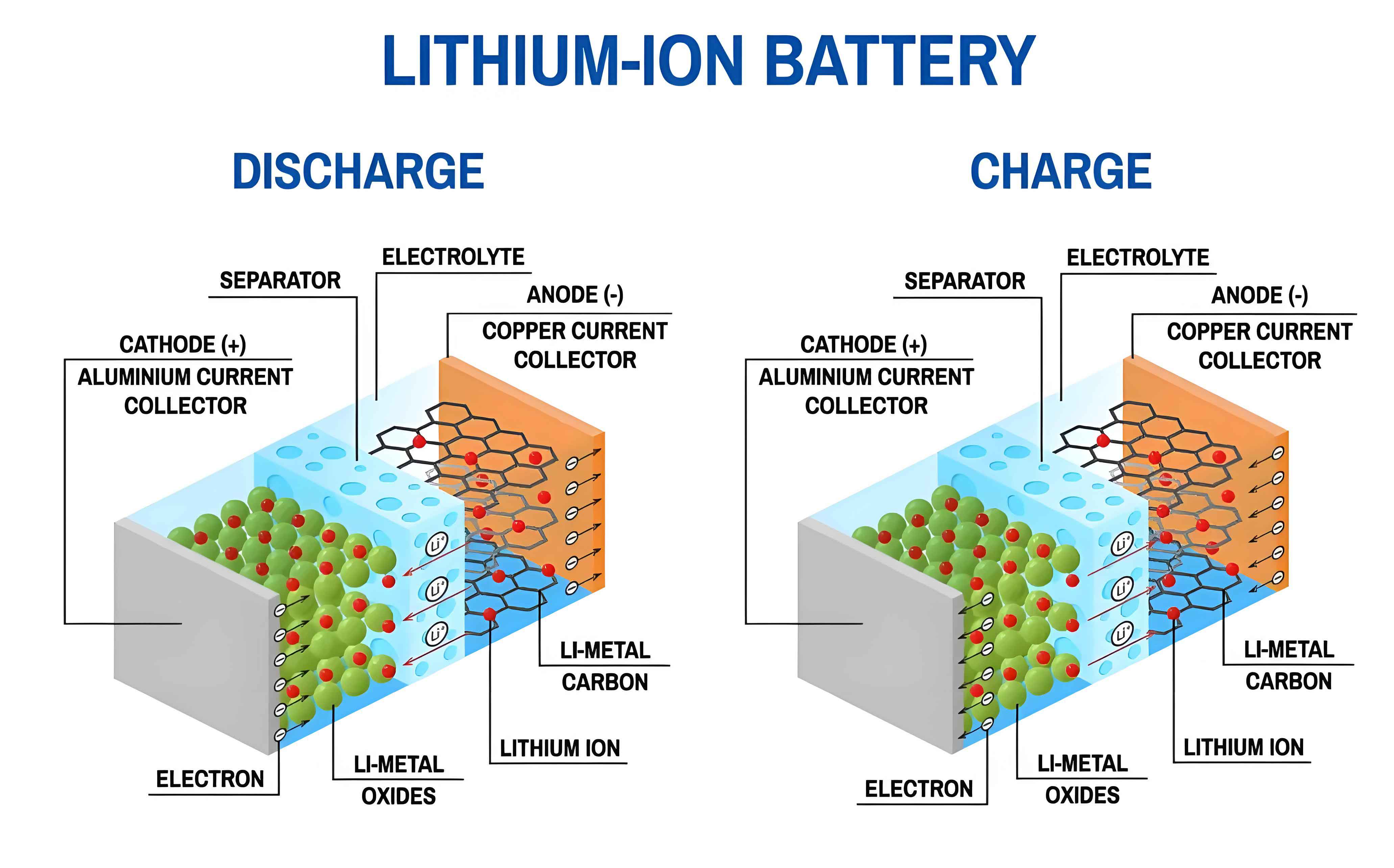
The development of sophisticated models for the lithium-ion battery is driven by the need to move beyond empirical correlations. While equivalent circuit models are computationally efficient and suitable for real-time state estimation in battery management systems, they lack the physical insight to extrapolate accurately to untested conditions or to predict internal phenomena like lithium plating or concentration gradients. Physics-based models, rooted in electrochemical principles, fill this gap. The most comprehensive of these is the Doyle-Fuller-Newman (DFN) model, also known as the pseudo-two-dimensional (P2D) model. It couples macroscopic transport through the porous electrode-separator stack with microscopic diffusion within active material particles.
The governing equations of the DFN model for a lithium-ion battery are summarized below. The model domain spans from the negative current collector (x=0) to the positive current collector (x=L), comprising the negative electrode (length Ln), separator (Ls), and positive electrode (Lp).
Solid-Phase Diffusion (in particle radius r):
$$ \frac{\partial c_s(r,x,t)}{\partial t} = \frac{1}{r^2} \frac{\partial}{\partial r} \left( D_s r^2 \frac{\partial c_s(r,x,t)}{\partial r} \right) $$
Boundary conditions:
$$ \left. D_s \frac{\partial c_s}{\partial r} \right|_{r=0} = 0; \quad \left. D_s \frac{\partial c_s}{\partial r} \right|_{r=R_p} = -\frac{j(x,t)}{F} $$
Liquid-Phase Diffusion and Migration (in through-thickness x):
$$ \frac{\partial c_e(x,t)}{\partial t} = \frac{\partial}{\partial x} \left( D_{e,\text{eff}} \frac{\partial c_e(x,t)}{\partial x} \right) + \frac{a(1-t_+^0)}{\epsilon_e} j(x,t) $$
Boundary conditions:
$$ \left. \frac{\partial c_e}{\partial x} \right|_{x=0, L} = 0 $$
Charge Conservation:
Solid phase:
$$ \frac{\partial}{\partial x} \left( \sigma_{s,\text{eff}} \frac{\partial \phi_s(x,t)}{\partial x} \right) = a F j(x,t) $$
Liquid phase:
$$ \frac{\partial}{\partial x} \left( \kappa_{\text{eff}} \frac{\partial \phi_e(x,t)}{\partial x} + \kappa_{D,\text{eff}} \frac{\partial \ln c_e(x,t)}{\partial x} \right) = -a F j(x,t) $$
with boundary conditions for potential gradients related to the applied current \(i_{app}(t)\).
Electrochemical Reaction Kinetics (Butler-Volmer Equation):
$$ j(x,t) = i_0(x,t) \left[ \exp\left(\frac{\alpha_a F}{RT}\eta(x,t)\right) – \exp\left(-\frac{\alpha_c F}{RT}\eta(x,t)\right) \right] $$
where the exchange current density is
$$ i_0(x,t) = k_{\text{eff}} F \left[c_e(x,t)\right]^{\alpha_a} \left[c_{s,\text{max}} – c_{s,s}(x,t)\right]^{\alpha_a} \left[c_{s,s}(x,t)\right]^{\alpha_c} $$
and the surface overpotential is
$$ \eta(x,t) = \phi_s(x,t) – \phi_e(x,t) – U(c_{s,s}(x,t)/c_{s,\text{max}}) – F R_f j(x,t) $$
Terminal Voltage:
$$ V(t) = \phi_s(L,t) – \phi_s(0,t) – \frac{R_{\text{cc}}}{A} i_{app}(t) $$
This system of coupled partial differential equations (PDEs) contains a significant number of parameters, each with physical meaning. Table 1 categorizes and lists the primary parameters for a standard DFN model of a lithium-ion battery.
| Category | Symbol | Description | Typical Unit |
|---|---|---|---|
| Geometric | \(L_n, L_s, L_p\) | Thickness of negative electrode, separator, positive electrode | m |
| \(A\) | Electrode cross-sectional area | m² | |
| \(\epsilon_{s,n}, \epsilon_{s,p}\) | Active material volume fraction (solid phase) | – | |
| \(\epsilon_{e,n}, \epsilon_{e,s}, \epsilon_{e,p}\) | Electrolyte phase porosity | – | |
| \(R_{p,n}, R_{p,p}\) | Radius of active material particles | m | |
| \(a_n, a_p\) | Specific interfacial area, \(a = 3\epsilon_s / R_p\) | m⁻¹ | |
| Transport | \(D_{s,n}, D_{s,p}\) | Solid-phase diffusion coefficient of Li⁺ | m²/s |
| \(D_e\) | Liquid-phase diffusion coefficient of Li⁺ | m²/s | |
| \(t_+^0\) | Li⁺ transference number | – | |
| \(\kappa\) | Electrolyte ionic conductivity | S/m | |
| Kinetic & Thermodynamic | \(k_n, k_p\) | Electrochemical reaction rate constant | m^{2.5}/(mol^{0.5}·s) |
| \(R_f\) | Film resistance (e.g., SEI) | Ω·m² | |
| \(U_n, U_p\) | Open-circuit potential (OCP) of electrode materials | V | |
| \(c_{s,\text{max},n}, c_{s,\text{max},p}\) | Maximum Li concentration in solid phase | mol/m³ | |
| \(c_{e,0}\) | Initial/bulk electrolyte concentration | mol/m³ | |
| Electrical | \(\sigma_{s,n}, \sigma_{s,p}\) | Solid-phase electronic conductivity | S/m |
| \(R_{\text{cc}}\) | Current collector contact resistance | Ω·m² |
Given the complexity and computational cost of solving the full DFN model, simplified models like the Single Particle Model (SPM) and the Single Particle Model with electrolyte (SPMe) are often employed for control-oriented applications or initial parameter studies. The SPM assumes each electrode behaves as a single spherical particle, neglecting electrolyte concentration gradients and potential variations. The SPMe adds a one-dimensional electrolyte model, offering a better balance between accuracy and computational load than the full DFN model for a lithium-ion battery.
The core challenge is that the values of these parameters are often unknown, variable with temperature and state-of-health (SoH), or difficult to measure directly. Parameter identification provides a solution. Before embarking on the computationally intensive optimization process, it is crucial to determine which parameters significantly influence the model output under the conditions of interest. This is the role of parameter sensitivity analysis (SA).
Sensitivity analysis methods are broadly classified into Local SA (LSA) and Global SA (GSA). LSA evaluates the effect of small perturbations of one parameter at a time around a nominal point. A simple derivative-based local sensitivity index \(S_j\) for a parameter \(\theta_j\) with respect to model output \(y\) is:
$$ S_j = \left| \frac{\partial y(\boldsymbol{\theta})}{\partial \theta_j} \right|_{\boldsymbol{\theta}=\boldsymbol{\theta}^*} $$
While computationally cheap (requiring \(n+1\) model runs for \(n\) parameters), LSA can be misleading for highly nonlinear systems like a lithium-ion battery model, as the sensitivity depends heavily on the chosen nominal point \(\boldsymbol{\theta}^*\) and ignores interactions between parameters.
A more robust variance-based LSA involves sampling the parameter \(\theta_j\) over a predefined plausible range \([\theta_j^{\text{min}}, \theta_j^{\text{max}}]\) while keeping others fixed, and computing the variance of the output:
$$ S_j^{\text{var}} = \text{Var}\left( y(\theta_j^i) \right) \quad \text{for} \quad i=1,…,N_s $$
This approach gives a better sense of the parameter’s influence across its possible range but remains an “one-at-a-time” method.
Global SA, in contrast, assesses the effect of varying all parameters simultaneously over their entire ranges, capturing interaction effects. The Morris method is a popular screening tool. It computes elementary effects \(EE_j^i\) for each parameter along randomized trajectories in the parameter space:
$$ EE_j^i = \frac{y(\theta_1, …, \theta_j + \Delta_j, …, \theta_n) – y(\boldsymbol{\theta})}{\Delta_j} $$
The mean \(\mu_j\) and standard deviation \(\sigma_j\) of the elementary effects across many trajectories are calculated. A high \(\mu_j\) indicates a parameter with large overall influence, while a high \(\sigma_j\) suggests nonlinear effects or interactions with other parameters.
The Sobol’ method is a more rigorous variance-based GSA. It decomposes the total variance of the output \(V(y)\) into contributions from individual parameters and their interactions:
$$ V(y) = \sum_j V_j + \sum_{j<k} $$<="" +="" …="" \sum_{j<k
It calculates first-order Sobol’ indices \(S_j = V_j / V(y)\), which measure the main effect of \(\theta_j\), and total-effect indices \(ST_j\), which measure the total contribution of \(\theta_j\) including all interactions. While accurate, Sobol’ analysis requires a large number of model evaluations (\(>1000\) for complex models), often necessitating the use of surrogate models.
The choice of SA method depends on the model complexity and computational budget. Table 2 summarizes the key characteristics and applicability of these methods for lithium-ion battery model analysis.
| Method | Type | Principle | Pros | Cons | Best For |
|---|---|---|---|---|---|
| Derivative-based | Local | Computes partial derivative at a nominal point. | Extremely fast; minimal simulations. | Only valid locally; misses interactions; sensitive to nominal point choice. | Initial screening of simple, near-linear models. |
| Variance-based (OAT) | Local | Computes output variance while varying one parameter over its range. | More robust than derivative method; accounts for parameter range. | Does not capture parameter interactions; results can be path-dependent. | Understanding individual parameter influence when interactions are weak. |
| Morris Method | Global Screening | Computes mean (µ) and std (σ) of elementary effects from multiple randomized OAT trajectories. | Relatively efficient; provides qualitative ranking and interaction insight (via σ). | Does not provide quantitative variance apportionment; screening tool only. | Identifying the subset of most influential parameters in complex models before detailed GSA. |
| Sobol’ Indices | Global Quantitative | Variance decomposition via Monte Carlo sampling. | Quantifies main and total effect contributions; captures all interactions. | Computationally very expensive; requires many model runs (>>1000). | Detailed, quantitative understanding of parameter importance and interactions for critical studies. |
Sensitivity analysis results for a lithium-ion battery model are highly dependent on the operating condition (e.g., C-rate, temperature), state-of-charge (SoC), and the specific output of interest (e.g., terminal voltage, cell temperature, overpotential). Therefore, SA should ideally be performed over the dynamic range of conditions relevant to the intended application of the identified model.
Once sensitive parameters are identified, the next step is parameter optimization or identification. This is formulated as a nonlinear least-squares minimization problem: find the parameter vector \(\boldsymbol{\theta}\) that minimizes the difference between the model output \(\hat{V}(t, \boldsymbol{\theta})\) and the experimentally measured voltage \(V_{\text{exp}}(t)\). A common objective function \(F(\boldsymbol{\theta})\) is the Root Mean Square Error (RMSE):
$$ F(\boldsymbol{\theta}) = \sqrt{ \frac{1}{N} \sum_{k=1}^{N} \left( \hat{V}(t_k, \boldsymbol{\theta}) – V_{\text{exp}}(t_k) \right)^2 } $$
More complex objective functions can incorporate multiple data types (e.g., voltage, temperature, expansion force) or different weighting for various SoC regions, especially important for flat-voltage lithium-ion battery chemistries like Lithium Iron Phosphate (LFP).
The optimization algorithms can be categorized into gradient-based and derivative-free (metaheuristic) methods. Gradient-based methods, like the Levenberg-Marquardt (LM) algorithm, use derivative information to quickly converge to a local minimum. The LM algorithm interpolates between the gradient descent and Gauss-Newton methods:
$$ \boldsymbol{\theta}_{k+1} = \boldsymbol{\theta}_k – \left[ \mathbf{J}^T\mathbf{J} + \lambda \text{diag}(\mathbf{J}^T\mathbf{J}) \right]^{-1} \mathbf{J}^T \mathbf{r}(\boldsymbol{\theta}_k) $$
where \(\mathbf{J}\) is the Jacobian matrix of residuals \(\mathbf{r}\), and \(\lambda\) is a damping parameter. While fast and accurate near a good initial guess, gradient-based methods can easily get trapped in local minima for the highly non-convex problem of lithium-ion battery parameter identification.
Metaheuristic algorithms are population-based stochastic search methods that do not require gradient information, making them robust for global optimization. Three prominent algorithms are:
1. Genetic Algorithm (GA): Inspired by natural selection. A population of candidate solutions (chromosomes) evolves over generations through selection, crossover, and mutation operators to minimize \(F(\boldsymbol{\theta})\).
2. Particle Swarm Optimization (PSO): Inspired by bird flocking. Particles move through the parameter space, with their velocity \(\mathbf{v}_i\) and position \(\mathbf{x}_i\) updated based on personal best (\(pbest_i\)) and global best (\(gbest\)) positions:
$$ \mathbf{v}_i^{k+1} = w \mathbf{v}_i^k + c_1 r_1 (pbest_i – \mathbf{x}_i^k) + c_2 r_2 (gbest – \mathbf{x}_i^k) $$
$$ \mathbf{x}_i^{k+1} = \mathbf{x}_i^k + \mathbf{v}_i^{k+1} $$
where \(w\) is inertia, \(c_1, c_2\) are acceleration coefficients, and \(r_1, r_2\) are random numbers.
3. Cuckoo Search (CS): Inspired by brood parasitism. New solutions \(\mathbf{x}_i\) are generated via Lévy flights, a type of random walk with heavy-tailed step lengths, enhancing global exploration:
$$ \mathbf{x}_i^{k+1} = \mathbf{x}_i^k + \alpha \oplus \text{Lévy}(\lambda) $$
A fraction of worse nests (solutions) are abandoned and replaced by new random ones, maintaining diversity.
Table 3 provides a comparative overview of these optimization algorithms in the context of lithium-ion battery parameter identification.
| Algorithm | Type | Key Mechanism | Advantages | Disadvantages |
|---|---|---|---|---|
| Levenberg-Marquardt (LM) | Gradient-based | Uses Jacobian; adaptively blends gradient descent and Gauss-Newton. | Very fast convergence near optimum; efficient for local refinement. | Requires derivative calculation/sensitivity; prone to converging to local minima; needs good initial guess. |
| Genetic Algorithm (GA) | Metaheuristic (Evolutionary) | Selection, crossover, mutation on a population of solutions. | Good global search capability; handles discrete/continuous variables; parallelizable. | Slow convergence; high computational cost per generation; many tuning parameters (rates, selection). |
| Particle Swarm Optimization (PSO) | Metaheuristic (Swarm Intelligence) | Particles follow personal and global best positions. | Conceptually simple; few parameters to tune; relatively fast convergence. | Can prematurely converge to local optima; performance sensitive to parameter settings (\(w, c_1, c_2\)). |
| Cuckoo Search (CS) | Metaheuristic (Swarm Intelligence) | Lévy flight global walk and elitist random local walk. | Few tuning parameters; Lévy flights enhance global exploration; often more efficient than GA/PSO. | Can be slower than PSO for some problems; requires careful setting of step size \(\alpha\) and discovery rate \(p_a\). |
In practice, a hybrid or multi-stage strategy is often most effective for lithium-ion battery parameter identification. For example, a global metaheuristic algorithm like CS or GA can be used first to locate a region near the global optimum, followed by a local gradient-based method like LM for precise refinement. Another common strategy is to decompose the problem: first identify capacity-related parameters (e.g., \(c_{s,\text{max}}\), electrode thicknesses) from low-rate discharge data, then identify kinetic and transport parameters (e.g., \(D_s\), \(k\)) from higher-rate or dynamic data with the capacity parameters fixed.
Future research directions in lithium-ion battery parameter identification are promising and multi-faceted. Firstly, the design of optimal experiments for identification is crucial. Not all test protocols excite all model parameters equally. Designing input current profiles (e.g., specific frequency content in pulses) that maximize the information content for the most uncertain parameters can significantly improve identifiability and reduce time/cost. Secondly, the integration of parameter identification with multi-physics and multi-scale models is essential. As models evolve to couple electrochemistry with thermal, mechanical, and aging phenomena, the parameter set expands dramatically. Identifying coupled parameters (e.g., temperature-dependent kinetics, stress-dependent diffusion) from multi-modal data (voltage, temperature, force) will be a key challenge. This necessitates advanced multi-objective optimization frameworks. Thirdly, the fusion with Artificial Intelligence (AI) offers transformative potential. Machine learning can be used to create accurate surrogate models (e.g., neural networks, Gaussian processes) that emulate the expensive physics-based model, making extensive SA and optimization runs feasible. Furthermore, AI can help analyze the temporal evolution of identified parameters to diagnose specific aging modes (e.g., SEI growth, lithium plating, particle cracking) in a data-driven yet physics-informed manner. Finally, moving towards online or adaptive identification frameworks, where model parameters are updated in real-time or periodically based on operational data from the battery management system, will be critical for enabling truly adaptive and predictive management of lithium-ion batteries throughout their lifecycle.
In conclusion, parameter identification is a cornerstone for the practical application of high-fidelity physics-based models for lithium-ion batteries. The workflow—from selecting an appropriate model, to analyzing parameter sensitivities, to executing a robust optimization—requires careful consideration of tools and strategies. While challenges remain in handling model complexity, parameter correlations, and computational cost, ongoing advancements in optimization algorithms, experimental design, and AI integration are steadily enhancing the robustness, efficiency, and scope of parameter identification techniques. This progress is vital for accelerating the design, improving the management, and extending the lifetime of lithium-ion batteries, thereby supporting the broader transition to sustainable energy systems.