
The rapid proliferation of renewable energy sources is fundamentally reshaping modern power systems, driving them towards a dual-high characteristic featuring a high proportion of renewables and a high penetration of power electronic devices. Large-scale solar photovoltaic (PV) farms and distributed small-scale PV systems are being integrated into the grid at an unprecedented rate. This integration often occurs via long transmission lines and transformers, creating a “weakly-connected” state between the generation sources and the main grid network, commonly referred to as a “weak grid.” The utility interactive inverter, serving as the critical interface between these renewable sources and the AC grid, is at the heart of this transformation. Its widespread integration, however, introduces complex stability challenges, significantly elevating the risk of wideband oscillations that threaten system reliability. To address these emerging challenges, impedance analysis has become an indispensable tool for investigating the interactive stability of grid-connected systems. This article provides a comprehensive review of the modeling methods for utility interactive inverters, analyzing their significance for system stability and outlining future research directions.
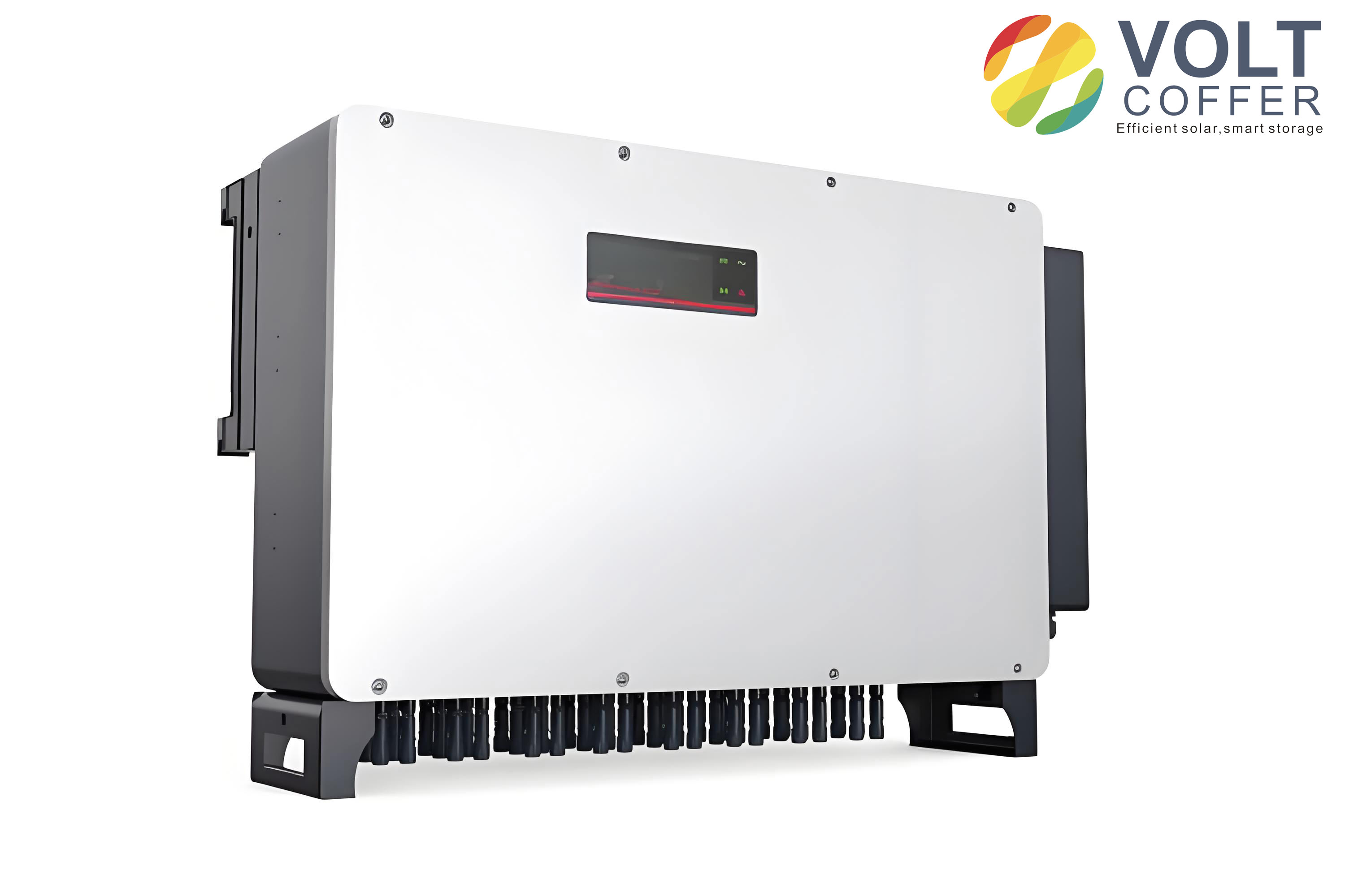
The stability and performance of a utility interactive inverter are intrinsically linked to the strength of the grid to which it is connected. Grid strength is commonly quantified by the Short-Circuit Ratio (SCR), defined as the ratio of the short-circuit capacity at the Point of Common Coupling (PCC) to the rated power of the inverter plant:
$$ \lambda_{SCR} = \frac{S_{sc}}{P} $$
A system with an SCR below 3 is generally considered a weak grid, and an SCR below 2 indicates an extremely weak grid where stability risks are severe. In such weak grid conditions, the impedance of the grid network becomes significant and interacts dynamically with the output impedance of the utility interactive inverter, potentially leading to harmonic resonance and instability across a wide frequency range.
Control Paradigms for Utility Interactive Inverters
The control strategy of a utility interactive inverter defines its external characteristics and its interaction with the grid. Two primary control paradigms have been established: grid-following (current-source mode) and grid-forming (voltage-source mode) control.
Grid-Following (Current-Source) Inverters: Traditionally, most utility interactive inverters operate in grid-following mode. They employ a Phase-Locked Loop (PLL) to synchronize with the grid voltage and behave as controlled current sources, injecting a current dictated by an internal reference. This control structure is effective in strong grids. However, in weak grids, the dynamics of the PLL can adversely interact with the grid impedance, leading to negative damping in the low-frequency range of the inverter’s output impedance. This interaction can destabilize the system, particularly if the PLL bandwidth is not carefully designed. The instability mechanisms are well-documented, showing that the stability margin decreases as grid impedance increases.
Grid-Forming (Voltage-Source) Inverters: To better support weak grids, grid-forming control strategies have gained significant attention. Instead of a PLL, these inverters often use power synchronization loops, such as those based on Virtual Synchronous Generator (VSG) or droop control principles, to establish the voltage frequency and amplitude. They present a voltage-source characteristic to the grid, mimicking the behavior of a traditional synchronous generator. This intrinsic characteristic makes the utility interactive inverter with grid-forming control more naturally compatible with weak grids, as its stability is less sensitive to high grid impedance. The effective SCR for a grid-forming inverter can be interpreted differently, often allowing stable operation even in very weak grid scenarios where grid-following inverters would fail.
The fundamental difference lies in their synchronization mechanism and the resulting terminal behavior. Grid-following inverters require a stable voltage to follow, while grid-forming inverters can establish and regulate the voltage themselves. This results in a complementary relationship: grid-following inverters are well-suited for strong grids, whereas grid-forming inverters offer superior stability in weak grids. The comparison is summarized in the table below.
| Feature | Grid-Following (Current-Source) Inverter | Grid-Forming (Voltage-Source) Inverter |
|---|---|---|
| Synchronization | Phase-Locked Loop (PLL) | Power/Frequency Droop, Virtual Inertia |
| External Characteristic | Controlled Current Source | Controlled Voltage Source |
| Stability in Strong Grid | Excellent | Good |
| Stability in Weak Grid | Challenging, prone to instability | Robust, inherently more stable |
| Primary Control Goal | Regulate output current/power | Regulate voltage magnitude and frequency |
The Critical Role of Impedance Modeling in Stability Analysis
Accurate modeling of the utility interactive inverter is the cornerstone for analyzing and ensuring system stability. The modeling approach directly influences the method used for stability assessment.
1. Significance for Stability Studies: Stability analysis can be broadly divided into large-disturbance (transient) stability and small-signal stability. Transient stability assesses the system’s ability to maintain synchronism after a major fault or disturbance. For a utility interactive inverter, this involves analyzing the nonlinear dynamic response of control loops, such as the power loop coupling and the influence of reactive power control on the power-angle characteristic. Small-signal stability, on the other hand, evaluates the system’s response to minor perturbations. This is crucial for identifying the onset of low-frequency oscillations and wideband resonances, which are prevalent in systems with high penetration of power electronics. A precise model allows for the identification of oscillatory modes, participation factors, and the root causes of instability.
2. Impedance Modeling for Wideband Oscillation Mitigation: Wideband electromagnetic oscillations, ranging from subsynchronous to supraharmonic frequencies, are a signature stability challenge in modern power-electronics-dominated systems. These oscillations arise from the dynamic interaction between the impedance of the grid and the impedance of the utility interactive inverter. Therefore, from an impedance perspective, the core of wideband oscillation analysis and suppression lies in understanding and shaping these impedances. The general principle for mitigation is to break the conditions for oscillation, which can be achieved by: (i) adding positive damping (resistance) to the system, (ii) shifting the controller bandwidths to avoid resonant frequency overlaps, or (iii) a combination of both. An accurate impedance model of the utility interactive inverter is, therefore, not just an analytical tool but a essential foundation for designing effective damping controls, harmonic filters, and robust control strategies that ensure stable integration under varying grid conditions.
| Stability Analysis Type | Focus | Modeling Requirement for Utility Interactive Inverter |
|---|---|---|
| Transient Stability | Large-disturbance response, fault ride-through, loss of synchronism. | Nonlinear, time-domain model to capture large-signal behavior of power/frequency controls. |
| Small-Signal Stability | Low-frequency oscillation, modal analysis, controller interaction. | Linearized state-space or impedance model around an operating point. |
| Harmonic/Wideband Stability | High-frequency resonance, stability under harmonic distortion. | Frequency-domain impedance model (e.g., dq or sequence domain). |
Impedance Modeling Methodologies for Utility Interactive Inverters
The construction of an accurate model for the utility interactive inverter is a prerequisite for stability analysis. Modeling methods can be categorized into time-domain and frequency-domain approaches. Time-domain methods, such as detailed switching simulations or state-space modeling, can be accurate but suffer from high computational burden or the “curse of dimensionality” for large systems. Frequency-domain methods, particularly impedance-based modeling, have become the preferred approach for analyzing interactive stability due to their modularity and physical intuitiveness.
The core idea of impedance-based stability assessment is to treat the utility interactive inverter and the grid as two interconnected subsystems. The inverter is represented by its Norton equivalent (a current source in parallel with an output admittance $Y_{inv}(s)$) or Thévenin equivalent (a voltage source in series with an output impedance $Z_{inv}(s)$). The grid is represented by its equivalent impedance $Z_g(s)$. The stability of the interconnected system can then be assessed using criteria like the Nyquist criterion based on the minor loop gain $L(s) = Z_g(s) Y_{inv}(s)$ or $Z_{inv}(s) / Z_g(s)$, depending on the representation. This modular approach allows for the independent modeling of the inverter; changes in its control only require updating its impedance model, not the entire system model.
1. Frequency-Domain Impedance Modeling
This is the most prevalent approach for harmonic stability analysis. The two main techniques are dq-domain linearization and harmonic linearization.
a) dq-Domain Impedance Modeling:
In this method, the three-phase AC quantities of the utility interactive inverter are transformed into the synchronous rotating dq-reference frame using the PLL angle. Under small-signal perturbation, the system is linearized, resulting in a 2×2 impedance matrix that describes the coupling between the d and q channels:
$$
\begin{bmatrix}
\Delta v_d(s) \\
\Delta v_q(s)
\end{bmatrix}
=
\begin{bmatrix}
Z_{dd}(s) & Z_{dq}(s) \\
Z_{qd}(s) & Z_{qq}(s)
\end{bmatrix}
\begin{bmatrix}
\Delta i_d(s) \\
\Delta i_q(s)
\end{bmatrix}
$$
Where $Z_{dd}, Z_{qq}$ are the direct impedances and $Z_{dq}, Z_{qd}$ are the cross-coupling impedances. This model naturally incorporates the dynamics of the PLL and current controllers. It is highly effective for analyzing low-frequency stability issues. The stability is assessed by examining the eigenvalues of the impedance ratio matrix or using a generalized Nyquist criterion for the multi-input multi-output (MIMO) system.
b) Harmonic Linearization (Sequence-Domain Impedance Modeling):
This method operates in the stationary sequence domain (positive-sequence and negative-sequence). It uses harmonic linearization theory to account for the frequency coupling effects inherent in synchronized utility interactive inverters. When a small-signal perturbation at frequency $f_p$ is injected, the nonlinearity of controllers like the PLL generates responses not only at $f_p$ but also at a coupled frequency $f_n$. This leads to a coupled impedance model:
$$
\begin{bmatrix}
\Delta V_p(s) \\
\Delta V_n(s)
\end{bmatrix}
=
\begin{bmatrix}
Z_{pp}(s) & Z_{pn}(s) \\
Z_{np}(s) & Z_{nn}(s)
\end{bmatrix}
\begin{bmatrix}
\Delta I_p(s) \\
\Delta I_n(s)
\end{bmatrix}
$$
Here, $Z_{pp}$ and $Z_{nn}$ are the self-impedances, while $Z_{pn}$ and $Z_{np}$ represent the coupling impedances between sequences. This model is crucial for accurately predicting stability in weak grids where frequency coupling is significant, especially in the subsynchronous and low-frequency range. It has been shown that ignoring these coupling terms ($Z_{pn}, Z_{np}$) can lead to inaccurate stability predictions.
2. State-Space Modeling
State-space modeling involves deriving the differential equations for all energy storage elements and dynamic states in the utility interactive inverter system, including the LCL filter inductors/capacitor, controller integrators, and PLL loops. The system is linearized around an operating point, resulting in a standard state-space form:
$$
\Delta \dot{\mathbf{x}} = \mathbf{A} \Delta \mathbf{x} + \mathbf{B} \Delta \mathbf{u}
$$
$$
\Delta \mathbf{y} = \mathbf{C} \Delta \mathbf{x} + \mathbf{D} \Delta \mathbf{u}
$$
Where $\Delta \mathbf{x}$ is the state vector, $\Delta \mathbf{u}$ is the input vector (e.g., grid voltage), and $\Delta \mathbf{y}$ is the output vector (e.g., inverter current). The system’s small-signal stability is determined by the eigenvalues of the state matrix $\mathbf{A}$; if any eigenvalue has a positive real part, the system is unstable. This method provides deep insight into modal interactions and allows for the calculation of participation factors to identify which states are most associated with a particular oscillatory mode. However, deriving a full-order model for a complex utility interactive inverter with multiple control loops is labor-intensive, and the model must be rebuilt if the system topology or control structure changes, making it less flexible for large-scale system studies compared to impedance methods.
3. Data-Driven and Neural Network-Based Impedance Identification
For complex or proprietary utility interactive inverters where an analytical white-box model is difficult to obtain, data-driven black-box or gray-box identification methods are valuable. These methods involve injecting perturbations into the operating inverter and measuring its response to identify its impedance characteristics. Recently, neural networks have been employed to build surrogate impedance models. For instance, a Radial Basis Function (RBF) neural network can be trained using data collected at various operating points and grid strengths. The inputs to the network can be frequency and grid SCR, while the outputs are the magnitude and phase of the sequence impedances (e.g., $Z_{pp}, Z_{pn}$). Once trained, this surrogate model can predict the impedance of the utility interactive inverter for any condition within the trained range, enabling rapid stability assessment without repeated analytical modeling or measurement. This approach is particularly promising for adapting to changing grid conditions and for the online stability monitoring of inverters with adaptive control.
| Modeling Method | Domain | Key Advantages | Key Challenges/Limitations |
|---|---|---|---|
| dq-Domain Impedance | Frequency (Rotating Frame) | Intuitively includes PLL/controller dynamics; standard for low-frequency analysis. | Requires careful handling of MIMO stability criteria; cross-coupling can complicate analysis. |
| Harmonic Linearization (Sequence) | Frequency (Stationary Frame) | Accurately captures frequency-coupling effects essential for weak-grid stability. | Model derivation is complex; results in higher-order impedance matrix. |
| State-Space | Time (Linearized) | Provides full modal analysis, participation factors; precise for given configuration. | Model derivation is tedious; not modular—entire model must be rebuilt for changes. |
| Neural Network Identification | Data-Driven / Frequency | Does not require internal knowledge; can adapt to varying conditions; good for online use. | Requires extensive training data; accuracy limited to training range; lacks physical insight. |
Advantages, Challenges, and Future Perspectives
The impedance-based modeling of utility interactive inverters offers distinct advantages that have solidified its role in modern power system analysis.
Advantages:
1. Modularity and Flexibility: The inverter and grid are modeled separately. Changes in the inverter’s control only necessitate updating its own impedance model, not the entire network model. This is invaluable for systems with many inverters.
2. Physical Intuition: The impedance model provides a clear frequency-domain representation of the inverter’s dynamic terminal behavior, making it easier to identify resonant points and design compatible controllers or filters.
3. Measurability: The impedance of an actual utility interactive inverter can be measured experimentally using perturbation injection techniques, even without knowledge of its internal control structure. This allows for model validation and black-box stability assessment.
4. Applicability to Wideband Stability: It is the most effective framework for analyzing harmonic resonance and wideband oscillation issues, which are difficult to tackle with traditional time-domain or state-space methods for large systems.
Persistent Challenges:
1. Model Complexity and Accuracy: Capturing all relevant dynamics, including nonlinear effects, frequency coupling, and the impact of various control loops (PLL, DC-link control, harmonic compensators) in a single accurate model remains challenging.
2. Time-Varying Parameters and Operating Points: The impedance of a utility interactive inverter can vary with operating point (e.g., power level, DC voltage). A model valid for one condition may not be accurate for another, requiring adaptive or parameter-varying models.
3. Multi-Inverter Interactions: Modeling the collective behavior of hundreds or thousands of inverters, considering their diverse control strategies and potential interactions, is an open area of research. Simplified aggregate models are needed but can obscure local instability phenomena.
4. Validation under Real Weak-Grid Conditions: Obtaining accurate impedance measurements in real weak grids with background distortion and fluctuating impedance is technically difficult.
Future Research Directions:
1. High-Fidelity, Unified Impedance Models: Developing more accurate models that seamlessly integrate the dynamics of both grid-following and grid-forming utility interactive inverters, including all ancillary services and fault response controls.
2. Impedance Modeling for Multi-Inverter Systems: Research into scalable impedance modeling and stability assessment methods for large clusters of inverters, including the development of practical aggregate impedance models.
3. AI-Enhanced Modeling and Stability Assessment: Leveraging machine learning and neural networks not only for identification but also for predicting stability boundaries, optimizing impedance shaping controls in real-time, and detecting emerging instability from operational data.
4. Cybersecurity and Robustness: Extending impedance-based analysis to evaluate the robustness of inverter controls against cyber-physical attacks or malicious grid disturbances.
5. Standardization and Tool Development: Promoting the standardization of impedance measurement procedures and the integration of advanced impedance-based stability analysis tools into commercial power system simulation software.
| Research Area | Current Challenge | Future Direction |
|---|---|---|
| Model Accuracy | Linearized models may miss key nonlinear dynamics and coupling effects. | Develop nonlinear impedance descriptors or hybrid linear/parameter-varying models. |
| System Scalability | Impedance-based analysis of systems with thousands of heterogeneous inverters is complex. | Create efficient aggregation methods and cloud/edge-computing platforms for system-wide stability monitoring. |
| Adaptive Control | Fixed impedance models are insufficient for inverters with self-tuning controls. | Integrate online impedance identification with adaptive control algorithms to maintain stability under all grid conditions. |
| New Technologies | Impedance models for emerging topologies (e.g., modular multilevel converters in PV plants) are less mature. | Extend harmonic linearization and modeling frameworks to new converter architectures and wide-bandgap semiconductor-based utility interactive inverters. |
In conclusion, impedance modeling has established itself as a fundamental and powerful paradigm for understanding and ensuring the stability of power systems increasingly dominated by utility interactive inverters. From the classical dq-domain models to the more sophisticated harmonic linearization approaches that capture essential weak-grid dynamics, the evolution of these methods has been driven by the practical needs of integrating renewable energy. While challenges remain in modeling complexity, scalability, and real-world validation, the future of this field is closely tied to advancements in data-driven techniques, standardized practices, and the development of robust, grid-forming control strategies. Continued research in impedance modeling is not merely an academic exercise but a critical engineering endeavor to enable the secure, reliable, and large-scale integration of renewable energy into the grid of the future.