
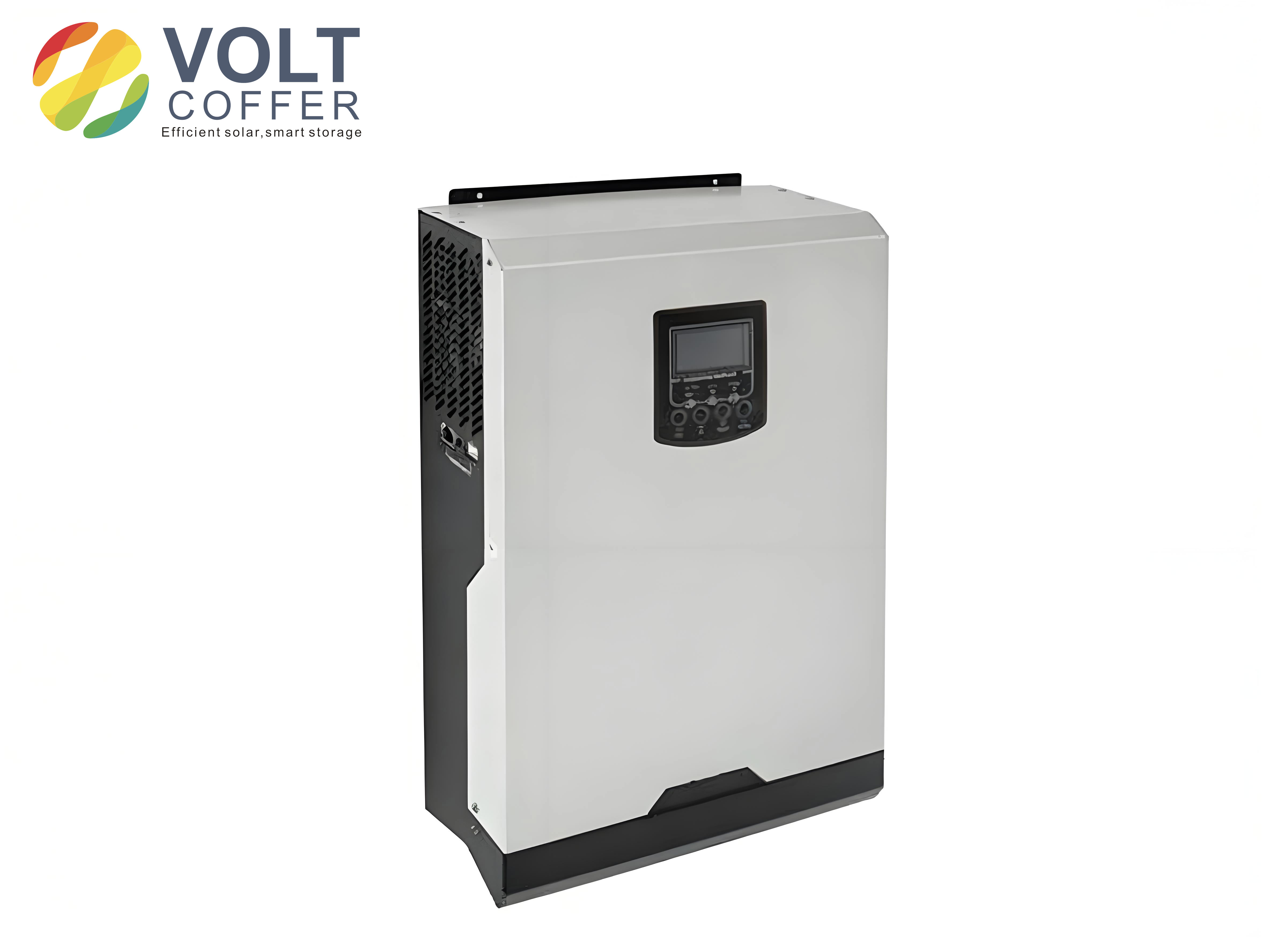
In this work I study a low-power solar inverter that connects a small photovoltaic array to a single-phase alternating-current grid. My main objective is to make the solar inverter operate with high efficiency, stable synchronization, and simple digital control. The system I designed uses a two-stage topology: a front-end boost converter for maximum power point tracking and a rear-end full-bridge inverter for grid-connected current injection. I focus on practical parameter selection, controller implementation, and experimental verification. Throughout the design process I treat the solar inverter as the central component that links the photovoltaic source to the utility network, because its behavior determines overall energy yield, output power quality, and protection performance.
1. Introduction and Design Motivation
The decreasing availability of coal, oil, and natural gas has made renewable energy essential for long-term sustainable development. Solar power is especially attractive because it is clean, widely distributed, and abundant. A grid-connected solar inverter eliminates the battery bank that is normally required in a stand-alone photovoltaic system. This reduces cost, system complexity, maintenance effort, and the energy losses associated with battery charging and discharging. For low-power residential or small commercial applications, a compact solar inverter with maximum power point tracking and reliable grid synchronization is therefore highly valuable.
I chose a two-stage architecture because it separates the maximum power point tracking task from the grid-connected inversion task. The front-end boost converter regulates the photovoltaic operating point and raises the direct-current voltage to a suitable level. The rear-end inverter converts the boosted direct-current voltage into a sinusoidal alternating-current current. This modular structure simplifies control and improves the flexibility of the solar inverter.
The main design targets of my low-power solar inverter are summarized in the following table.
| Parameter | Value | Remark |
|---|---|---|
| Rated input direct-current voltage | 400 V | Boost converter output |
| Maximum power point tracking range | 140 V to 180 V | Photovoltaic array voltage |
| Rated output alternating-current voltage | 220 V root mean square | Single-phase grid |
| Rated output frequency | 50 Hz | Grid frequency |
| Rated output power | 500 W | Low-power solar inverter |
| Power factor requirement | Greater than 0.95 | Near-unity power factor |
| Output current total harmonic distortion | Less than 5% | Grid current quality |
2. Photovoltaic Cell Model and Output Characteristics
The photovoltaic cell converts solar radiation into electrical energy through the photovoltaic effect of a semiconductor p-n junction. When photons with sufficient energy strike the junction, electron-hole pairs are generated. The internal electric field separates these carriers, producing a photocurrent and a terminal voltage. A practical photovoltaic cell can be represented by a current source in parallel with a diode, a shunt resistance, and a series resistance.
The terminal current of a photovoltaic cell can be written as
$$
I = I_{ph} – I_0 \left[ \exp\left( \frac{q(U + I R_s)}{A k T} \right) – 1 \right] – \frac{U + I R_s}{R_{sh}}
$$
where \(I_{ph}\) is the photocurrent, \(I_0\) is the diode saturation current, \(q\) is the electron charge, \(U\) is the terminal voltage, \(I\) is the terminal current, \(R_s\) is the series resistance, \(R_{sh}\) is the shunt resistance, \(A\) is the diode ideality factor, \(k\) is Boltzmann’s constant, and \(T\) is the absolute temperature.
For an ideal photovoltaic cell, the series resistance is very small and the shunt resistance is very large. Therefore, the simplified model becomes
$$
I = I_{ph} – I_0 \left[ \exp\left( \frac{qU}{A k T} \right) – 1 \right]
$$
The output power is
$$
P = U I
$$
At a constant temperature and irradiance, there is a unique maximum power point on the power-voltage curve. The maximum power point tracking algorithm must keep the solar inverter operating at or very close to this point. The standard test condition is usually defined as an irradiance of \(1000 \, \mathrm{W/m^2}\), a cell temperature of \(25^\circ\mathrm{C}\), and an air mass of \(1.5\).
I built a simulation model of the photovoltaic array in a Simulink environment. The model accepts irradiance and temperature as inputs and produces current, voltage, and power outputs. The simulation confirms that the short-circuit current is approximately proportional to irradiance, while the open-circuit voltage decreases as temperature rises. The maximum output power increases with irradiance and decreases with temperature.
| Condition | Observed Effect on Photovoltaic Output |
|---|---|
| Irradiance increases | Short-circuit current increases; maximum power increases |
| Irradiance decreases | Short-circuit current decreases; maximum power decreases |
| Temperature increases | Open-circuit voltage decreases; maximum power decreases |
| Temperature decreases | Open-circuit voltage increases; maximum power increases |
| Load resistance changes | Operating point moves along the current-voltage curve |
3. Maximum Power Point Tracking Methods
Because the photovoltaic source is nonlinear, maximum power point tracking is essential for a high-performance solar inverter. I compared several classical methods before selecting the algorithm used in my design. The main candidates are constant voltage tracking, perturb and observe, incremental conductance, and fuzzy duty-cycle perturbation.
3.1 Constant Voltage Tracking
Constant voltage tracking assumes that the maximum power point voltage remains approximately constant when temperature does not vary significantly. The control target is simply to hold the photovoltaic voltage near a preset value. This method is simple and inexpensive, but it does not respond well to large temperature changes. It is suitable only for applications with limited temperature variation.
3.2 Perturb and Observe
In perturb and observe, the controller periodically changes the duty cycle or voltage and observes the resulting power. If the power increases, the next perturbation continues in the same direction. If the power decreases, the perturbation direction is reversed. This method is easy to implement and requires only voltage and current measurements. However, it oscillates around the maximum power point and can misjudge the direction under rapidly changing irradiance.
3.3 Incremental Conductance
The incremental conductance method uses the fact that the derivative of power with respect to voltage is zero at the maximum power point:
$$
\frac{dP}{dU} = \frac{d(UI)}{dU} = I + U \frac{dI}{dU} = 0
$$
Therefore,
$$
\frac{dI}{dU} = – \frac{I}{U}
$$
If \(\frac{dI}{dU} > – \frac{I}{U}\), the operating point is to the left of the maximum power point and the voltage should increase. If \(\frac{dI}{dU} < – \frac{I}{U}\), the operating point is to the right and the voltage should decrease. This method provides good steady-state accuracy, but it is more complex and can fail during sudden irradiance changes.
3.4 Fuzzy Duty-Cycle Perturbation
To overcome the limitations of conventional perturb and observe, I applied a fuzzy logic controller to the duty-cycle perturbation method. The fuzzy controller uses the power change and the previous duty-cycle step as inputs and produces the next duty-cycle step as output. I define the power change \(\Delta P\) and duty-cycle step \(A\) as fuzzy sets.
$$
\Delta P = \{ NB, NM, NS, N0, P0, PS, PM, PB \}
$$
$$
A = \{ NB, NM, NS, PS, PM, PB \}
$$
The corresponding universes of discourse are
$$
\Delta P = \{-6,-5,-4,-3,-2,-1,-0,+0,+1,+2,+3,+4,+5,+6\}
$$
$$
A = \{-6,-5,-4,-3,-2,-1,+1,+2,+3,+4,+5,+6\}
$$
I used triangular membership functions for simplicity and practical implementation. The fuzzy rule base adjusts the duty-cycle step according to the power change. A representative rule table is shown below.
| Power Change \(\Delta P\) | Previous Step NB | Previous Step NM | Previous Step NS | Previous Step PS | Previous Step PM | Previous Step PB |
|---|---|---|---|---|---|---|
| NB | NB | NB | NM | NS | NS | PS |
| NM | NB | NB | NM | NS | PS | PS |
| NS | NB | NM | NS | PS | PS | PM |
| N0 | NM | NS | NS | PS | PM | PM |
| P0 | NM | NS | PS | PS | PM | PM |
| PS | NS | NS | PS | PM | PM | PB |
| PM | NS | PS | PM | PM | PB | PB |
| PB | PS | PM | PM | PB | PB | PB |
The fuzzy controller output is defuzzified to obtain the duty-cycle increment. The updated duty cycle is
$$
D(n) = D(n-1) + \Delta D(n)
$$
I tested this method in simulation. When the irradiance was \(1000 \, \mathrm{W/m^2}\), the fuzzy duty-cycle perturbation reached a stable power of approximately \(64 \, \mathrm{W}\) in about \(0.03 \, \mathrm{s}\). When the irradiance changed to \(800 \, \mathrm{W/m^2}\) at \(0.4 \, \mathrm{s}\), the controller reached a new stable power of about \(49 \, \mathrm{W}\) in approximately \(0.01 \, \mathrm{s}\). This fast tracking response is a major advantage for a solar inverter operating under variable sunlight.
| Method | Advantages | Disadvantages |
|---|---|---|
| Constant voltage tracking | Simple, low cost | Poor temperature response |
| Perturb and observe | Easy, few sensors | Oscillation, possible misjudgment |
| Incremental conductance | Good steady-state accuracy | Complex, sensitive to rapid changes |
| Fuzzy duty-cycle perturbation | Fast, robust, reduced oscillation | Requires rule design and tuning |
4. Front-End Boost Converter Design
The front-end boost converter performs maximum power point tracking and raises the photovoltaic voltage to the direct-current bus voltage required by the solar inverter. I selected a boost topology because it has a continuous input current, which is favorable for photovoltaic sources, and because its voltage gain can be controlled easily through the duty cycle.
In continuous conduction mode, the ideal voltage conversion ratio is
$$
\frac{V_{dc}}{V_{pv}} = \frac{1}{1-D}
$$
where \(V_{dc}\) is the direct-current bus voltage, \(V_{pv}\) is the photovoltaic voltage, and \(D\) is the duty cycle. For my design, the maximum photovoltaic voltage is approximately \(140 \, \mathrm{V}\) and the direct-current bus voltage is \(400 \, \mathrm{V}\). Therefore, the maximum duty cycle is
$$
D_{max} = 1 – \frac{V_{pv,min}}{V_{dc}} = 1 – \frac{140}{400} = 0.65
$$
The peak-to-peak inductor current ripple is
$$
\Delta i_L = \frac{V_{pv} D T_s}{L}
$$
To keep the converter in continuous conduction mode and to limit the current ripple, I calculated the inductor value. A practical design equation for the minimum inductance is
$$
L \geq \frac{4 V_{dc}^2 T_s}{27 P_{RL} \eta}
$$
Using a switching frequency of \(200 \, \mathrm{kHz}\), a current ripple ratio of \(25\%\), and a rated output power of \(500 \, \mathrm{W}\), I obtained an inductance of approximately \(9.48 \, \mathrm{mH}\). I selected \(10 \, \mathrm{mH}\) to provide margin.
The output capacitor must limit the direct-current bus voltage ripple. The capacitor requirement can be estimated as
$$
C \geq \frac{P_{RL} D T_s}{V_{dc} \Delta V_{dc}}
$$
With a voltage ripple limit of \(1\%\), the calculated capacitance was about \(10.16 \, \mu\mathrm{F}\). I selected a larger capacitance of \(110 \, \mu\mathrm{F}\) to improve voltage stability. In the actual circuit, two \(220 \, \mu\mathrm{F}\) capacitors rated at \(250 \, \mathrm{V}\) were connected in series to obtain an equivalent capacitance of \(110 \, \mu\mathrm{F}\) with a higher voltage rating.
| Boost Converter Parameter | Symbol | Calculated or Selected Value |
|---|---|---|
| Input voltage range | \(V_{pv}\) | 140 V to 180 V |
| Direct-current bus voltage | \(V_{dc}\) | 400 V |
| Maximum duty cycle | \(D_{max}\) | 0.65 |
| Switching frequency | \(f_s\) | 200 kHz |
| Inductor | \(L\) | 10 mH |
| Output capacitor | \(C\) | 110 \(\mu\)F |
| Power switch | \(VT\) | 600 V, 9 A MOSFET |
| Diode | \(VD\) | 600 V, 8 A fast recovery diode |
I selected a power MOSFET with a voltage rating of \(600 \, \mathrm{V}\) and a current rating of \(9 \, \mathrm{A}\). The diode was chosen as a fast recovery diode with a reverse voltage rating of \(600 \, \mathrm{V}\), an average forward current of \(8 \, \mathrm{A}\), and a recovery time below \(30 \, \mathrm{ns}\). These ratings provide sufficient margin for the low-power solar inverter.
5. Rear-End Inverter Design
The rear-end stage is a single-phase full-bridge voltage-source inverter. It converts the direct-current bus voltage into a sinusoidal alternating-current current that is synchronized with the grid. The full-bridge inverter contains four controlled switches and four antiparallel diodes. The antiparallel diodes provide a path for reactive power and help maintain current continuity.
I used an LC low-pass filter at the inverter output. The filter attenuates the high-frequency switching harmonics produced by the solar inverter while allowing the fundamental grid frequency to pass with minimal distortion. The filter inductor is designed from the current ripple requirement:
$$
L = \frac{U_{om}(U_{dc} – U_{om})}{\Delta i_L U_{dc}} T
$$
where \(U_{om}\) is the peak output voltage, \(U_{dc}\) is the direct-current bus voltage, \(\Delta i_L\) is the allowable current ripple, and \(T\) is the switching period. I set the allowable current ripple to \(18\%\) of the rated current. With an output power of \(500 \, \mathrm{W}\), an efficiency of \(96\%\), and an output voltage of \(220 \, \mathrm{V}\), the maximum current ripple was approximately \(0.43 \, \mathrm{A}\). The calculated inductance was about \(8.05 \, \mathrm{mH}\). I selected \(10 \, \mathrm{mH}\) with a rated current of \(6 \, \mathrm{A}\) to improve filtering and provide margin.
The LC resonance frequency must be well below the switching frequency and well above the fundamental frequency:
$$
f_1 \ll f_c \ll f_s
$$
A practical rule is
$$
10 f_1 < f_c < \frac{1}{10} f_s
$$
For a fundamental frequency of \(50 \, \mathrm{Hz}\) and a switching frequency of \(20 \, \mathrm{kHz}\), I selected a cutoff frequency near \(1.6 \, \mathrm{kHz}\). The filter capacitance was calculated from
$$
f_c = \frac{1}{2\pi\sqrt{LC}}
$$
Using \(L = 7.62 \, \mathrm{mH}\) and \(C = 0.832 \, \mu\mathrm{F}\), the cutoff frequency was close to the desired value. In the final design I used \(L = 10 \, \mathrm{mH}\) and a corresponding capacitance that satisfied the harmonic attenuation requirement.
The transfer function of the LC filter is
$$
G(s) = \frac{U_o(s)}{U_i(s)} = \frac{\omega_L^2}{s^2 + 2\zeta\omega_L s + \omega_L^2}
$$
where \(\omega_L = 12560 \, \mathrm{rad/s}\) and \(\zeta = 0.5\). The Bode plot of this filter shows that frequencies below approximately \(350 \, \mathrm{rad/s}\) pass with little attenuation, while harmonics above \(410 \, \mathrm{rad/s}\) are suppressed. This meets the filtering requirements of the solar inverter.
| Inverter Filter Parameter | Symbol | Value |
|---|---|---|
| Rated output power | \(P_o\) | 500 W |
| Output voltage | \(U_o\) | 220 V root mean square |
| Peak output voltage | \(U_{om}\) | 311 V |
| Switching frequency | \(f_s\) | 20 kHz |
| Filter inductor | \(L\) | 10 mH |
| Filter capacitor | \(C\) | 0.832 \(\mu\)F |
| Cutoff frequency | \(f_c\) | Approximately 1.6 kHz |
6. Auxiliary Power, Sampling, and Protection Circuits
A practical solar inverter requires auxiliary supplies for control, sampling, and gate driving. I designed a multi-output auxiliary power supply using a switching regulator. The input was taken from the direct-current bus in the range of \(140 \, \mathrm{V}\) to \(180 \, \mathrm{V}\), and the outputs were \(+3 \, \mathrm{V}\), \(+15 \, \mathrm{V}\), and \(-15 \, \mathrm{V}\). The output ripple was kept below \(1\%\).
The auxiliary supply used a flyback topology with an RCD snubber to suppress voltage spikes caused by leakage inductance. A precision shunt regulator and an optocoupler were used in the feedback path to regulate the output voltage. The optocoupler provides galvanic isolation between the output side and the control side, which improves noise immunity and safety.
For voltage and current sensing, I used Hall-effect sensors. The direct-current bus voltage was measured with a voltage Hall sensor whose output current is converted to a voltage by a measuring resistor. The signal was then filtered, buffered, and clamped before being sent to the analog-to-digital converter of the digital signal processor. The analog input range of the processor is \(0 \, \mathrm{V}\) to \(3 \, \mathrm{V}\), so I limited the signal to approximately \(2.5 \, \mathrm{V}\) for safety.
The grid voltage phase was obtained by a zero-crossing detection circuit. The grid voltage was stepped down, filtered, and compared with a reference to produce a square wave. The rising edge of this square wave corresponds to the positive-going zero crossing of the grid voltage. This signal was connected to the capture input of the digital signal processor for phase locking.
The output current was measured with a Hall-effect current sensor. The measured signal was conditioned by a follower, an amplifier, and a limiting circuit. This provided a safe analog signal for the current control loop of the solar inverter.
| Signal | Sensor Type | Conditioning | Processor Interface |
|---|---|---|---|
| Direct-current bus voltage | Voltage Hall sensor | Filter, buffer, clamp | ADC input |
| Direct-current bus current | Current Hall sensor | Filter, buffer, clamp | ADC input |
| Grid voltage phase | Zero-crossing comparator | Step-down, filter, square wave | Capture input |
| Output current | Current Hall sensor | Follower, amplifier, clamp | ADC input |
The gate drive circuit was based on a high-voltage gate driver integrated circuit. It provides independent high-side and low-side outputs and supports bootstrap operation for the high-side switch. The bootstrap capacitor was selected to supply the gate charge required by the power MOSFET. The bootstrap diode was a fast recovery diode to minimize charge loss and to block the high direct-current voltage.
I also designed overcurrent and overvoltage protection circuits. When the measured signal exceeds a preset threshold, the protection circuit sends a fault signal to the digital signal processor. The processor then immediately disables the pulse-width modulation outputs. This hardware protection operates independently of the software and improves the safety of the solar inverter.
7. Control Strategy for the Grid-Connected Solar Inverter
I used a double closed-loop control strategy based on sinusoidal pulse-width modulation. The outer loop regulates the direct-current bus voltage, and the inner loop regulates the output current. The outer voltage loop compares the measured direct-current bus voltage with a reference. The error is processed by a proportional-integral controller to produce a current amplitude command. This command is multiplied by a sinusoidal signal synchronized with the grid voltage to generate the reference current.
The inner current loop compares the actual output current with the reference current. The current error is processed by another proportional-integral controller. A grid voltage feedforward term is added to reduce the control effort and improve dynamic response. The resulting signal is compared with a triangular carrier to generate the sinusoidal pulse-width modulation signals for the four switches of the full-bridge inverter.
The outer voltage loop equation can be expressed as
$$
i_{ref} = K_{pv} (U_{dc}^* – U_{dc}) + K_{iv} \int (U_{dc}^* – U_{dc}) dt
$$
The inner current loop equation is
$$
u_{ctrl} = K_{pi} (i_{ref} – i_o) + K_{ii} \int (i_{ref} – i_o) dt + u_{grid}
$$
where \(U_{dc}^*\) is the reference direct-current bus voltage, \(i_{ref}\) is the reference current, \(i_o\) is the output current, \(u_{grid}\) is the grid voltage feedforward signal, and \(u_{ctrl}\) is the control signal for pulse-width modulation.
This double-loop strategy provides fast current tracking and stable direct-current bus voltage regulation. The current loop forces the output current to follow the grid voltage waveform, while the voltage loop maintains the power balance between the photovoltaic array and the grid. The feedforward term reduces the burden on the feedback controller and helps achieve near-unity power factor.
| Control Loop | Controlled Variable | Main Function |
|---|---|---|
| Outer voltage loop | Direct-current bus voltage | Stabilizes bus voltage and generates current amplitude |
| Inner current loop | Output alternating current | Tracks reference current and shapes waveform |
| Phase-locked loop | Grid phase | Synchronizes output current with grid voltage |
| Maximum power point tracking | Photovoltaic duty cycle | Extracts maximum available solar power |
I simulated the complete solar inverter with the double closed-loop controller. The simulation included the photovoltaic array model, the boost converter, the full-bridge inverter, the LC filter, and the grid connection. When the irradiance changed from \(1000 \, \mathrm{W/m^2}\) to \(800 \, \mathrm{W/m^2}\) at \(1 \, \mathrm{s}\), the output current showed a short transient and then settled to a new steady-state amplitude. The output current remained sinusoidal and approximately in phase with the grid voltage.
8. Digital Implementation on the DSP
The digital controller of my solar inverter was implemented on a fixed-point digital signal processor. The processor provides fast computation, multiple pulse-width modulation channels, analog-to-digital converters, capture units, and event managers. The software performs analog sampling, maximum power point tracking, sinusoidal pulse-width modulation generation, phase locking, filtering, and fault handling.
8.1 Pulse-Width Modulation Generation
The event manager contains general-purpose timers and full compare units. I used a continuous up-down counting mode to generate symmetrical pulse-width modulation. In this mode, the timer counts from zero to the period register and then back to zero. The compare register determines the duty cycle. The period register determines the switching frequency.
The switching period is
$$
T = \frac{2 \cdot T1PR}{f_{clock}}
$$
The duty cycle is
$$
D = \frac{T1PR – T1CMPR}{T1PR}
$$
for active-high output, or
$$
D = \frac{T1CMPR}{T1PR}
$$
for active-low output. By updating the compare register, I can change the duty cycle of the solar inverter in real time.
8.2 Sinusoidal Pulse-Width Modulation
I used an asymmetric regular sampling method for sinusoidal pulse-width modulation. The modulation wave is sampled at the positive and negative peaks of the triangular carrier. The switching instants are calculated from the sampled values. The pulse width is
$$
t_{on} = \frac{T_c}{2} + \frac{T_c M}{4} \left( \sin\frac{2\pi k}{N} – \sin\frac{2\pi(k+1)}{N} \right)
$$
where \(T_c\) is the carrier period, \(M\) is the modulation index, \(k\) is the sampling index, and \(N\) is the carrier-to-modulation frequency ratio. This method approximates natural sampling closely and is suitable for real-time digital implementation. I used a carrier frequency of \(20 \, \mathrm{kHz}\) and a modulation frequency of \(50 \, \mathrm{Hz}\), giving a frequency ratio of \(400\).
8.3 Maximum Power Point Tracking Program
The maximum power point tracking routine runs periodically in a timer interrupt. It samples the photovoltaic voltage and current, computes the power, and updates the duty cycle according to the fuzzy duty-cycle perturbation algorithm. The control flow is simple: measure, compute power change, evaluate fuzzy rules, update the duty cycle, and return.
The power change is computed as
$$
\Delta P = P(n) – P(n-1)
$$
The duty-cycle update is
$$
D(n) = D(n-1) + \Delta D(n)
$$
where \(\Delta D(n)\) is the fuzzy controller output. I limited the duty cycle to a safe range to prevent the boost converter from entering an unstable region. The maximum power point tracking routine also includes protection logic to stop the solar inverter if the input voltage or current exceeds safe limits.
8.4 Digital Filtering
The analog-to-digital converter samples are affected by switching noise and external interference. I used a combination of median filtering and arithmetic averaging. For each measurement, the controller takes multiple samples, removes the maximum and minimum values, and averages the remaining samples. The filtered value is
$$
y = \frac{1}{n-2} \sum_{k=1}^{n} x_k
$$
where the maximum and minimum samples are excluded. This method suppresses impulsive noise and random fluctuations while maintaining acceptable response speed.
| Filtering Method | Principle | Suitable Application |
|---|---|---|
| Program judgment | Reject samples exceeding a deviation limit | Occasional pulse noise |
| Median filter | Sort samples and take the middle value | Slowly varying signals |
| Arithmetic average | Average multiple samples | Random noise |
| Moving average | Average a sliding window | Periodic noise |
| Median plus average | Remove extremes and average | Direct-current signals in solar inverter |
8.5 Software Phase Locking
To connect the solar inverter to the grid, the output current must be synchronized with the grid voltage in both frequency and phase. I implemented a software phase-locked loop using the capture unit. The grid voltage zero-crossing signal is connected to the capture input, and the capture interrupt measures the grid period. The controller adjusts the pulse-width modulation period register to match the grid frequency. It also adjusts the index of the sine lookup table to correct the phase error.
If the output current leads the grid voltage, the sine table pointer is decreased to delay the output. If the output current lags the grid voltage, the pointer is increased to advance the output. The phase error is corrected in small steps, and the steady-state phase error is limited to one table step. This method is simple, robust, and easy to implement in the solar inverter software.
8.6 Anti-Interference Measures
Digital controllers in power electronic systems are exposed to strong electromagnetic interference. I used several measures to improve software reliability. Hardware shielding, isolation, and filtering reduce the entry of noise. In software, I placed unused interrupt vectors with trap routines and used the watchdog timer of the processor. If the program runs away or enters an infinite loop, the watchdog timer is not refreshed and generates a reset. This returns the solar inverter to a safe state and improves long-term reliability.
9. Experimental Results and Discussion
I built a laboratory prototype of the low-power solar inverter to verify the design. The prototype included the boost converter, the full-bridge inverter, the gate drive circuits, the sampling circuits, and the digital controller. The front-end boost converter was tested first. The pulse-width modulation output from the analog controller had a frequency of approximately \(27.17 \, \mathrm{kHz}\), which is close to the designed value of \(27 \, \mathrm{kHz}\). The waveform was clean with only small spikes.
The rear-end inverter was then tested with a resistive load. The sinusoidal pulse-width modulation signal from the digital processor was isolated and amplified by the gate driver. The measured switching frequency was approximately \(19.55 \, \mathrm{kHz}\), which is close to the designed \(20 \, \mathrm{kHz}\). The output voltage waveform showed acceptable sinusoidal shape, although some distortion appeared near the peaks under certain load conditions.
| Test Item | Designed Value | Measured Value | Observation |
|---|---|---|---|
| Boost converter switching frequency | 27 kHz | 27.17 kHz | Close to design |
| Inverter switching frequency | 20 kHz | 19.55 kHz | Close to design |
| Direct-current bus voltage | 400 V | Approximately 400 V | Stable with ripple |
| Output voltage | 220 V root mean square | Approximately 220 V | Distortion near peaks |
| Output frequency | 50 Hz | Approximately 50 Hz | Synchronized |
| Output current total harmonic distortion | Less than 5% | Near limit | Improved by filtering |
The experimental results show that the main functions of the solar inverter were achieved. The boost converter tracked the maximum power point, the inverter produced a sinusoidal output, and the digital controller maintained synchronization with the grid. The remaining distortion was caused by switching noise, dead time, and nonideal filtering. These effects can be reduced by improving the filter design, increasing the control loop bandwidth, and optimizing the printed circuit board layout.
10. Conclusions
I designed and studied a low-power solar inverter for grid-connected photovoltaic applications. The system uses a two-stage topology: a boost converter for maximum power point tracking and a full-bridge inverter for grid-connected power conversion. I developed a photovoltaic array model, compared several maximum power point tracking algorithms, and selected a fuzzy duty-cycle perturbation method for fast and stable tracking. I calculated the main parameters of the boost converter and the inverter filter, designed the auxiliary power supply, sampling circuits, gate drive circuits, and protection circuits, and implemented the control algorithms on a digital signal processor.
The key contributions of my work can be summarized as follows. First, I used a two-stage structure that separates maximum power point tracking from grid-connected inversion, making the solar inverter easier to control and optimize. Second, I applied a fuzzy logic controller to the duty-cycle perturbation method, which reduced oscillation and improved tracking speed under changing irradiance. Third, I implemented a double closed-loop control strategy with voltage outer loop and current inner loop, achieving stable direct-current bus voltage and sinusoidal output current. Fourth, I used software phase locking to synchronize the output current with the grid voltage, which is essential for a grid-connected solar inverter.
The experimental results confirmed that the designed solar inverter can operate with the intended functions. The switching frequencies were close to the design values, the direct-current bus voltage was stable, and the output current was approximately synchronized with the grid voltage. The output waveform quality was acceptable for a low-power prototype, although further work is needed to reduce harmonic distortion and improve efficiency.
11. Future Work
Several improvements can extend this research. The maximum power point tracking performance can be studied under partial shading conditions, where multiple local maxima may appear. A more advanced global optimization algorithm could be combined with the fuzzy controller. The front-end boost converter can be controlled directly by the digital signal processor instead of an analog controller, which would allow full digital integration of the solar inverter. Electromagnetic interference can be analyzed and reduced through better layout, shielding, and filter design. Finally, islanding detection and anti-islanding protection should be added to meet grid interconnection standards for a commercial solar inverter.
In summary, my research shows that a low-power solar inverter with fuzzy maximum power point tracking and double closed-loop control is feasible, practical, and suitable for small-scale distributed photovoltaic generation. The solar inverter remains the key enabling component for efficient and reliable grid connection, and continued improvements in its control and power stage will directly increase the value of solar energy systems.