
In modern power systems, the integration of renewable energy sources, particularly photovoltaic (PV) generation, has become pivotal. However, PV power generation is inherently intermittent and susceptible to environmental factors such as weather variations, leading to sudden fluctuations in the DC-side bus voltage of utility interactive inverters. These disturbances can compromise grid stability, cause voltage sags or swells, and in severe cases, trigger system collapse. As a researcher deeply involved in power electronics and grid integration, I have focused on enhancing the robustness and performance of utility interactive inverters. The core challenge lies in effectively managing reactive power and voltage control under dynamic grid conditions. Traditional control methods often fall short in handling rapid disturbances due to their reliance on precise system models and limited adaptability. In this paper, I propose a novel auto-disturbance rejection control (ADRC) strategy that synergistically combines frequency-domain identification and disturbance observation techniques. This approach aims to fortify the utility interactive inverter against voltage instabilities by actively estimating and compensating for internal and external perturbations, thereby ensuring safe and stable operation of the power system. The utility interactive inverter, as a critical interface between PV arrays and the grid, must exhibit high resilience to maintain power quality and support grid ancillary services. My methodology leverages a detailed mathematical model of the utility interactive inverter, incorporates a disturbance observer for real-time perturbation estimation, and employs frequency-domain identification to tailor the control response, ultimately achieving superior reactive power and voltage regulation.
The foundation of my control strategy is a comprehensive mathematical model of the utility interactive inverter. Typically, a three-phase voltage-source inverter topology is employed, interfacing the PV DC source with the AC grid via an LCL filter to attenuate switching harmonics. The dynamics of the utility interactive inverter are governed by both the DC-link and AC-side equations. On the DC side, the power balance involves the PV output, the inverter input, and the losses across the DC-link capacitor and parasitic resistance. The active power consumed by the DC-link capacitor \(C\) and resistance \(R\) is given by:
$$ P = \frac{C}{2} \frac{dU_{dc}^2}{dt} + \frac{U_{dc}^2}{R} $$
where \(U_{dc}\) is the DC bus voltage, and \(P\) represents the net active power flowing into the inverter. For the AC side, considering the filter inductance \(L\), the differential equations in the stationary \(\alpha\beta\) frame are:
$$ L \frac{di_{f\alpha}}{dt} = e_{f\alpha} – u_{f\alpha} $$
$$ L \frac{di_{f\beta}}{dt} = e_{f\beta} – u_{f\beta} $$
Here, \(i_{f\alpha}\) and \(i_{f\beta}\) are the \(\alpha\beta\)-axis components of the inductor current, \(e_{f\alpha}\) and \(e_{f\beta}\) denote the inverter output voltage components, and \(u_{f\alpha}\) and \(u_{f\beta}\) represent the grid voltage components. To facilitate control design, I transform these equations into the synchronous rotating \(dq\) frame aligned with the grid voltage vector. This transformation decouples the active and reactive power components, which are primarily controlled by the \(d\)-axis and \(q\)-axis currents, respectively. The state-space representation of the utility interactive inverter in the \(dq\) frame is:
$$ \frac{di_d}{dt} = -\frac{R}{L} i_d + \omega i_q + \frac{1}{L} (e_d – u_d) $$
$$ \frac{di_q}{dt} = -\frac{R}{L} i_q – \omega i_d + \frac{1}{L} (e_q – u_q) $$
where \(i_d\) and \(i_q\) are the \(dq\)-axis currents, \(e_d\) and \(e_q\) are the inverter voltage components, \(u_d\) and \(u_q\) are the grid voltage components, \(R\) is the filter resistance, and \(\omega\) is the grid angular frequency. The reactive power \(Q\) and active power \(P\) injected into the grid relate to these currents as \(P = \frac{3}{2}(u_d i_d + u_q i_q)\) and \(Q = \frac{3}{2}(u_q i_d – u_d i_q)\), assuming grid voltage orientation with \(u_q = 0\). Thus, regulating \(i_q\) directly influences the reactive power flow and, consequently, the voltage at the point of common coupling (PCC). The utility interactive inverter must maintain precise control over \(i_q\) to support voltage stability, especially during grid disturbances.
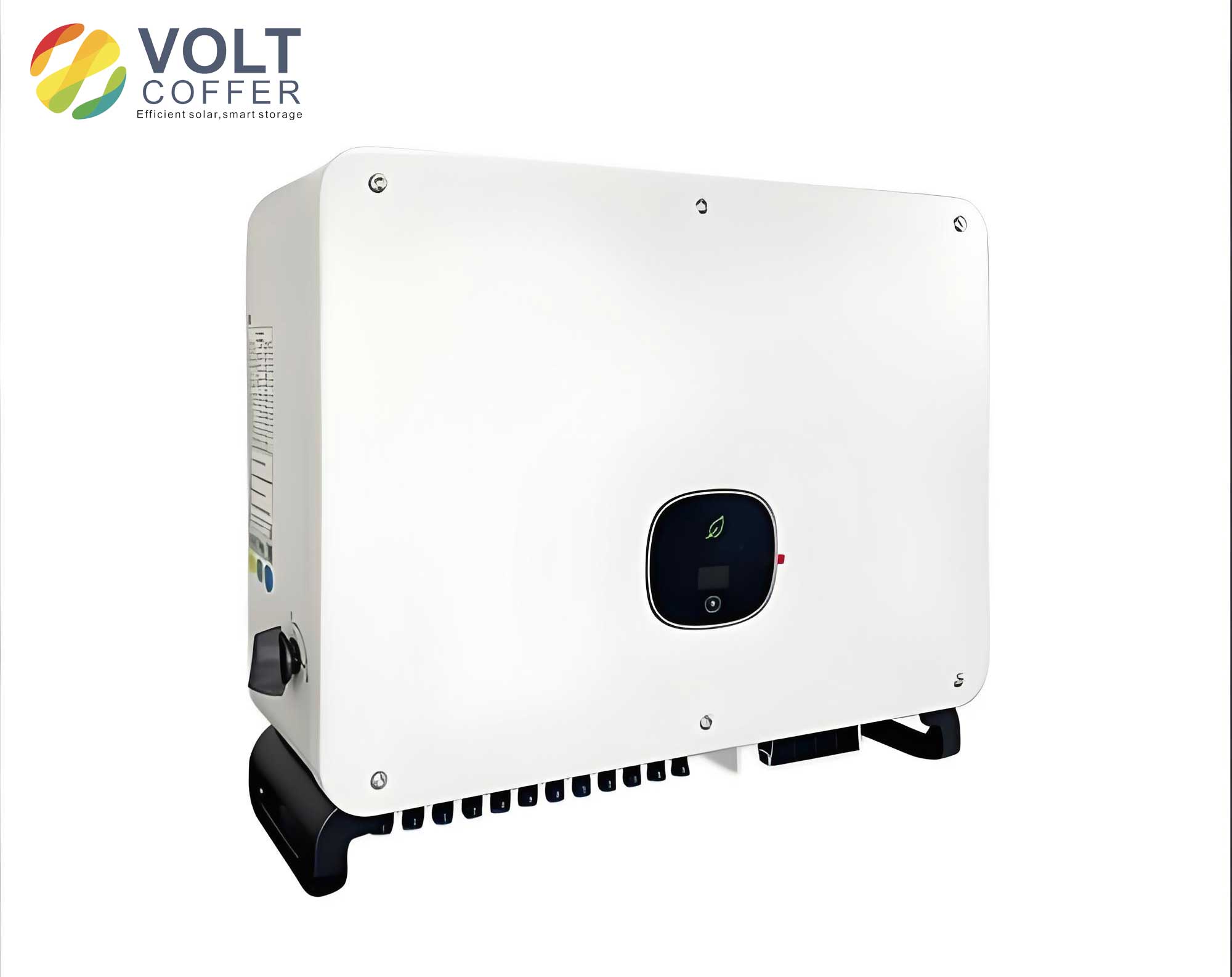
To address the vulnerability of the utility interactive inverter to disturbances, I incorporate a disturbance observer (DOB) into the control architecture. The DOB estimates the lumped disturbances affecting the system, which include model uncertainties, parameter variations, and external grid perturbations. For the current control loop, the disturbance \(d\) encompasses terms such as cross-coupling voltages, grid voltage harmonics, and unmodeled dynamics. The observer is designed based on the nominal model of the utility interactive inverter. Let the nominal plant transfer function be \(G_n(s)\), and the actual plant be \(G(s) = G_n(s) + \Delta G(s)\), where \(\Delta G(s)\) represents model deviations. The DOB estimates the disturbance \(\hat{d}\) using the control input \(u\) and the measured output \(y\). The structure of the DOB is:
$$ \hat{d} = Q(s) \left[ G_n^{-1}(s) y – u \right] $$
where \(Q(s)\) is a low-pass filter with a cutoff frequency selected to ensure robust estimation while attenuating measurement noise. The estimated disturbance \(\hat{d}\) is then fed forward to compensate the control input, yielding a modified control law \(u = u_{fb} – \hat{d}\), where \(u_{fb}\) is the output of the feedback controller. This effectively linearizes the system and enhances its disturbance rejection capability. For the utility interactive inverter, applying the DOB to the \(q\)-axis current loop helps mitigate reactive power fluctuations caused by grid voltage sags or swells. The observer dynamics can be expressed in state-space form for digital implementation. Consider the \(q\)-axis current dynamics with disturbance:
$$ L \frac{di_q}{dt} = e_q – u_q + d_q $$
where \(d_q\) aggregates all disturbances affecting the \(q\)-axis. A state observer can be constructed as:
$$ \frac{d\hat{i}_q}{dt} = \frac{1}{L} (e_q – u_q + \hat{d}_q) + k_o (i_q – \hat{i}_q) $$
$$ \frac{d\hat{d}_q}{dt} = \gamma (i_q – \hat{i}_q) $$
Here, \(\hat{i}_q\) is the estimated current, \(\hat{d}_q\) is the estimated disturbance, and \(k_o\), \(\gamma\) are observer gains tuned for fast convergence. The utility interactive inverter benefits significantly from this observer, as it enables real-time compensation of voltage disturbances without requiring precise knowledge of grid impedance or operating points.
While the disturbance observer handles low-frequency perturbations, the utility interactive inverter also faces challenges from resonant frequencies introduced by the LCL filter and grid interactions. To address this, I integrate frequency-domain identification techniques to characterize the system’s impedance and adapt the control parameters accordingly. Frequency-domain identification involves injecting a small-signal perturbation signal (e.g., a pseudo-random binary sequence or sinusoidal sweep) into the control loop and measuring the response of the utility interactive inverter. From the input-output data, I estimate the frequency response function (FRF), which reveals the system’s gain and phase characteristics across a spectrum. This is crucial for identifying resonant peaks that may lead to instability. The identified FRF can be used to refine the controller design, particularly for the ADRC structure. The auto-disturbance rejection controller for the utility interactive inverter combines the DOB with a state feedback mechanism that actively rejects disturbances estimated via frequency-domain insights. The ADRC framework treats all uncertainties as an extended state, which is estimated and canceled. For the \(q\)-axis voltage control, I define the system states as \(x_1 = i_q\), \(x_2 = \dot{i}_q\), and \(x_3 = f_d\), where \(f_d\) represents the total disturbance. The state equations are:
$$ \dot{x}_1 = x_2 $$
$$ \dot{x}_2 = x_3 + b u $$
$$ \dot{x}_3 = h $$
where \(b\) is a control gain derived from the nominal model, and \(h\) is the derivative of the disturbance. An extended state observer (ESO) is designed to estimate \(x_1\), \(x_2\), and \(x_3\):
$$ \dot{\hat{x}}_1 = \hat{x}_2 + \beta_1 (x_1 – \hat{x}_1) $$
$$ \dot{\hat{x}}_2 = \hat{x}_3 + b u + \beta_2 (x_1 – \hat{x}_1) $$
$$ \dot{\hat{x}}_3 = \beta_3 (x_1 – \hat{x}_1) $$
The observer gains \(\beta_1\), \(\beta_2\), \(\beta_3\) are selected to place the observer poles appropriately, ensuring rapid and accurate estimation. The control law is then:
$$ u = \frac{u_0 – \hat{x}_3}{b} $$
where \(u_0\) is the output of a linear state feedback controller, e.g., \(u_0 = k_p (i_{q}^* – \hat{x}_1) – k_d \hat{x}_2\), with \(i_{q}^*\) being the reactive current reference. The frequency-domain identification informs the tuning of \(k_p\), \(k_d\), and the observer gains by providing insights into the system’s phase margin and bandwidth limitations. For instance, if the identification reveals a resonance at a specific frequency, the controller can be augmented with a notch filter or the gains can be adjusted to dampen oscillations. This adaptive tuning is vital for the utility interactive inverter to maintain stability across varying grid conditions.
To validate the proposed ADRC strategy for the utility interactive inverter, I conducted extensive simulation studies using a detailed model in a power systems software environment. The test bench comprised a 100-kW PV system connected to a 380-V three-phase grid via a utility interactive inverter with an LCL filter. The key parameters are summarized in Table 1.
| Parameter | Value |
|---|---|
| Grid Voltage (line-to-line) | 380 V |
| Rated Active Power | 100 kW |
| DC-Link Capacitance | 1100 µF |
| Filter Inductance (L) | 2 mH |
| Filter Capacitance (Cf) | 50 µF |
| Switching Frequency | 10 kHz |
| Observer Gains (β1, β2, β3) | 0.2, 0.05, 0.01 |
| Control Gains (kp, kd) | 5, 0.1 |
The performance of the utility interactive inverter under the proposed ADRC was compared against conventional proportional-integral (PI) control and a vector control method with decoupling. The evaluation metrics included disturbance rejection, robustness to parameter variations, and steady-state voltage regulation. First, I tested the response to a sudden grid voltage dip—a common disturbance for utility interactive inverters. At time t = 0.2 s, the grid voltage amplitude dropped to 80% of its nominal value. The reactive current reference was set to 20 A to support voltage recovery. The results, quantified in Table 2, demonstrate the superiority of the ADRC approach.
| Control Method | Maximum Current Deviation (A) | Recovery Time (cycles) | Overshoot Voltage (V) |
|---|---|---|---|
| Proposed ADRC | 4.5 | 0.5 | 2.9 |
| Conventional PI | 15.2 | 2.0 | 8.7 |
| Vector Control | 12.8 | 1.8 | 7.5 |
The utility interactive inverter with ADRC exhibited minimal deviation and rapid recovery within half a grid cycle, highlighting its enhanced anti-disturbance capability. This is attributed to the effective estimation and compensation of grid voltage perturbations by the disturbance observer. In contrast, conventional methods showed prolonged oscillations and larger overshoots, which could stress the inverter components and degrade power quality. The utility interactive inverter must often operate under uncertain parameters due to aging, temperature variations, or manufacturing tolerances. To assess robustness, I performed a Monte Carlo analysis with 300 random trials, where the filter inductance and capacitance values varied by ±10% from their nominal values. The reactive current reference underwent a step change at t = 0.1 s. The statistical outcomes are presented in Table 3.
| Control Method | Mean Current Error (A) | Standard Deviation (A) | Stability Rate (%) |
|---|---|---|---|
| Proposed ADRC | 0.15 | 0.08 | 100 |
| Conventional PI | 1.23 | 0.45 | 85 |
| Vector Control | 0.98 | 0.32 | 88 |
The ADRC-based utility interactive inverter maintained stable operation in all trials, with negligible current error and low dispersion, confirming its robustness. The frequency-domain identification played a key role here by enabling adaptive tuning of the observer gains to accommodate parameter shifts. For instance, the identified resonance frequency of the LCL filter varied across trials, but the controller adjusted its damping accordingly, preventing harmonic instability. This adaptability is crucial for utility interactive inverters deployed in diverse grid environments.
Steady-state performance is equally vital for the utility interactive inverter, as it affects long-term power quality and compliance with grid codes. I evaluated the voltage regulation during load transients. Initially, the inverter operated at no-load, and then a resistive load was switched on and off at voltage peaks. The voltage total harmonic distortion (THD) and dynamic response were measured. Table 4 summarizes the results for a load step change from 0% to 100% rated power.
| Control Method | Voltage Sag Depth (V) | Recovery Time (ms) | THD at Steady-State (%) |
|---|---|---|---|
| Proposed ADRC | 2.3 | 25 | 0.75 |
| Conventional PI | 5.8 | 50 | 3.45 |
| Vector Control | 4.9 | 42 | 2.89 |
The utility interactive inverter with ADRC demonstrated superior voltage support, with a shallow sag and quick recovery, keeping THD well below the 3% limit. The disturbance observer effectively compensated for load-induced voltage drops, while the frequency-domain identification ensured that the control bandwidth did not excite filter resonances. This synergy between observation and identification is a hallmark of my approach, setting it apart from traditional methods. To further illustrate the control dynamics, I derive the closed-loop transfer function for the q-axis current under ADRC. Assuming perfect disturbance estimation (\(\hat{x}_3 = x_3\)), the system reduces to a double integrator with feedback. The transfer function from reference \(i_q^*\) to actual \(i_q\) is:
$$ G_{cl}(s) = \frac{k_p}{s^2 + k_d s + k_p} $$
This second-order system can be tuned for critical damping by setting \(k_d = 2\sqrt{k_p}\), ensuring fast response without overshoot. However, in practice, the utility interactive inverter faces delays and non-idealities. The frequency-domain identification helps refine these gains by providing phase margin data. For example, if the identified phase margin at the gain crossover frequency is low, \(k_p\) can be reduced to enhance stability. This iterative tuning process, facilitated by real-time identification, makes the utility interactive inverter adaptable to changing grid conditions.
The implementation of the proposed ADRC for a utility interactive inverter involves several practical considerations. Digital signal processors (DSPs) are typically used for real-time control, with sampling frequencies in the range of 10-20 kHz. The disturbance observer and ESO algorithms must be discretized for digital execution. Using the forward Euler method, the discrete-time ESO equations become:
$$ \hat{x}_1[k+1] = \hat{x}_1[k] + T_s \left( \hat{x}_2[k] + \beta_1 (i_q[k] – \hat{x}_1[k]) \right) $$
$$ \hat{x}_2[k+1] = \hat{x}_2[k] + T_s \left( \hat{x}_3[k] + b u[k] + \beta_2 (i_q[k] – \hat{x}_1[k]) \right) $$
$$ \hat{x}_3[k+1] = \hat{x}_3[k] + T_s \beta_3 (i_q[k] – \hat{x}_1[k]) $$
where \(T_s\) is the sampling period. The utility interactive inverter’s control loop thus operates with minimal computational overhead, as the ESO requires only a few multiplications and additions per cycle. Moreover, the frequency-domain identification can be run periodically or triggered during steady-state intervals to update controller parameters, ensuring continuous optimization. This adaptability is particularly beneficial for utility interactive inverters in microgrids or weak grids, where impedance varies frequently due to switching events or distributed generation fluctuations.
In conclusion, my research presents a robust auto-disturbance rejection control strategy for utility interactive inverters, integrating frequency-domain identification and disturbance observation. The methodology addresses key challenges in reactive power and voltage regulation, offering enhanced disturbance rejection, robustness to parameter uncertainties, and superior steady-state performance. The utility interactive inverter, as a frontline device in renewable energy integration, benefits from this approach through improved grid support capabilities and resilience against voltage instabilities. Future work will explore hardware-in-the-loop validation and extension to multi-inverter systems for coordinated voltage control. By advancing the control paradigms for utility interactive inverters, we can pave the way for more stable and efficient power networks in the era of sustainable energy.