
The global energy landscape is undergoing a transformative shift towards sustainability, driven by the urgent need to mitigate climate change and reduce reliance on fossil fuels. Renewable energy sources, particularly solar photovoltaic (PV) and wind power, have seen exponential growth in installed capacity. In many regions, these sources are now integral parts of the power grid, often connected through power electronic interfaces such as grid-tied inverters. A grid-tied inverter is a critical component that converts DC power from renewable sources into AC power synchronized with the utility grid. The widespread adoption of grid-tied inverters has led to the emergence of modern power systems with high penetration of inverter-based resources. However, this integration introduces new challenges, especially during grid faults. Unlike traditional synchronous generators, which have inherent inertial response and well-understood fault current characteristics, grid-tied inverters exhibit controlled and limited fault behavior. This discrepancy can affect the operation of conventional protection relays, potentially leading to maloperation and system instability. Therefore, a comprehensive study of the fault characteristics of power systems with grid-tied inverters is essential to ensure reliable and secure grid operation.
The three-phase grid-tied inverter is typically used in medium to large-scale PV systems. Its topology includes a DC source (e.g., PV array), a three-phase voltage-source inverter (VSI), a DC-link capacitor, an LCL filter, and a grid connection point. The LCL filter is crucial for reducing switching harmonics and ensuring compliance with grid standards. The grid-tied inverter operates by modulating the DC voltage into AC waveforms that match the grid’s frequency and phase. During normal operation, the grid-tied inverter controls the power flow to meet setpoints for active and reactive power. However, during faults, the control strategies must adapt to limit currents and provide grid support as required by regulations.
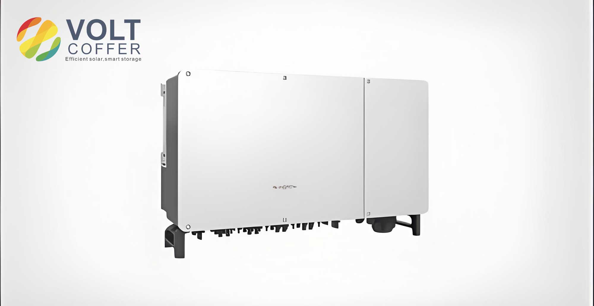
Mathematically, the dynamics of a grid-tied inverter can be modeled in the synchronous rotating dq reference frame. This transformation simplifies the control design by converting AC quantities into DC components. The voltage equations are as follows:
$$ u_d = L \frac{di_d}{dt} + R i_d + \omega_1 L i_q + u_{gd} $$
$$ u_q = L \frac{di_q}{dt} + R i_q – \omega_1 L i_d + u_{gq} $$
In these equations, the terms represent the inverter output voltage, the voltage drop across the filter impedance, and the grid voltage. The cross-coupling terms \( \omega_1 L i_q \) and \( -\omega_1 L i_d \) arise from the reference frame rotation and are compensated in advanced control schemes. Here, \( u_d \) and \( u_q \) are the d-axis and q-axis components of the inverter output voltage, \( i_d \) and \( i_q \) are the d-axis and q-axis components of the inverter output current, \( u_{gd} \) and \( u_{gq} \) are the d-axis and q-axis components of the grid voltage, \( L \) is the equivalent inductance of the filter, \( R \) is the equivalent resistance, and \( \omega_1 \) is the angular frequency of the grid voltage. This model forms the basis for designing control strategies for the grid-tied inverter.
The most common control strategy for grid-tied inverters is the PQ control, which enables independent control of active and reactive power. This strategy uses a cascaded control structure with an inner current loop and an outer power loop. The inner current loop ensures fast tracking of current references, while the outer power loop generates these references based on power setpoints. The current loop controllers are typically proportional-integral (PI) regulators, expressed in the Laplace domain as:
$$ G_c(s) = k_1 + \frac{k_2}{s} $$
Thus, the current dynamics become:
$$ L \frac{di_d}{dt} = \left( k_1 + \frac{k_2}{s} \right) (i_{d\_ref} – i_d) $$
$$ L \frac{di_q}{dt} = \left( k_1 + \frac{k_2}{s} \right) (i_{q\_ref} – i_q) $$
The reference currents \( i_{d\_ref} \) and \( i_{q\_ref} \) are derived from the power loop, which also uses PI controllers:
$$ i_{d\_ref} = \left( k_3 + \frac{k_4}{s} \right) (P_{out\_ref} – P_{out}) $$
$$ i_{q\_ref} = \left( k_3 + \frac{k_4}{s} \right) (Q_{out\_ref} – Q_{out}) $$
The active and reactive power outputs are calculated from the measured currents and voltages. Assuming grid voltage orientation where the d-axis aligns with the voltage vector, we have \( u_{gq} = 0 \), so:
$$ P_{out} = u_{gd} i_d = U_g i_d $$
$$ Q_{out} = -u_{gd} i_q = -U_g i_q $$
This simplification is common in control design for grid-tied inverters. The parameters \( k_1, k_2, k_3, k_4 \) are tuned to achieve desired performance, such as fast response and stability. The following table summarizes typical control parameters for a grid-tied inverter.
| Parameter | Symbol | Typical Value | Description |
|---|---|---|---|
| Proportional Gain (Inner Loop) | \( k_1 \) | 0.1 – 1.0 | Determines response speed |
| Integral Gain (Inner Loop) | \( k_2 \) | 10 – 100 | Eliminates steady-state error |
| Proportional Gain (Outer Loop) | \( k_3 \) | 0.01 – 0.1 | Slower response for power control |
| Integral Gain (Outer Loop) | \( k_4 \) | 1 – 10 | Integrates power error |
When a short-circuit fault occurs in the grid, the voltage at the point of common coupling (PCC) drops significantly. This voltage dip causes a surge in current from the grid-tied inverter if not properly controlled. To protect the inverter and other equipment, current limiting is implemented. There are two primary methods: passive limiting using resistors and inductors, and active limiting through control algorithms. In passive limiting, series inductors increase the impedance, while parallel resistors dissipate energy, thereby reducing the fault current. Active limiting involves modifying the PWM signals to clamp the output current to a safe maximum value. Both methods are essential for ensuring the durability of the grid-tied inverter during faults.
Furthermore, grid codes mandate that grid-tied inverters must have low-voltage ride-through (LVRT) capability. This means that during a voltage dip, the inverter should remain connected to the grid and inject reactive current to help restore voltage. The LVRT profile specifies the required behavior based on the voltage level. For example, when the voltage drops between 20% and 90% of nominal, the inverter must inject reactive current proportional to the voltage deviation. The mathematical representation is given by:
$$
I_T =
\begin{cases}
k_1 (0.9 – U_{g1}) I_g & \text{if } 0.2 \leq U_{g1} \leq 0.9 \\
k_2 I_g & \text{if } U_{g1} < 0.2 \\
0 & \text{if } U_{g1} > 0.9
\end{cases}
$$
with the constraint \( I_T \leq I_{max} \). Here, \( U_{g1} \) is the per-unit voltage at PCC, \( I_g \) is the rated current, and \( k_1, k_2 \) are constants typically greater than 1.5 and 1.05, respectively. The LVRT capability ensures that grid-tied inverters contribute to grid stability during disturbances rather than exacerbating them by disconnecting. The following table outlines the LVRT requirements for grid-tied inverters.
| Voltage Range (p.u.) | Reactive Current Requirement | Duration |
|---|---|---|
| 0.2 to 0.9 | \( I_T \geq k_1 (0.9 – U_{g1}) I_g \) | 0.15 s continuous |
| Below 0.2 | \( I_T \geq k_2 I_g \) | Until voltage recovery |
| Above 0.9 | No requirement | N/A |
In asymmetric faults, where voltage unbalance occurs, the control of positive and negative sequence currents becomes important. The grid-tied inverter can be controlled to inject balanced currents or to provide specific support. Using symmetric component theory, the reference currents in the dq frame for positive and negative sequences are derived. The general form is:
$$
\begin{bmatrix}
i^*_{1d} \\
i^*_{1q} \\
i^*_{2d} \\
i^*_{2q}
\end{bmatrix}
=
\begin{bmatrix}
u_{1d} & u_{1q} \\
u_{1q} & -u_{1d} \\
-K u_{2d} & K u_{2q} \\
-K u_{2q} & -K u_{2d}
\end{bmatrix}
\begin{bmatrix}
\frac{P^*_0}{M} \\
\frac{Q^*_0}{N}
\end{bmatrix}
$$
where \( K \) is a parameter that determines the control objective. For instance, \( K = 0 \) eliminates negative sequence current, \( K = -1 \) minimizes reactive power oscillations, and \( K = 1 \) minimizes active power oscillations. The terms \( M \) and \( N \) are normalization factors defined as:
$$ M = u_{1d}^2 + u_{1q}^2 – K u_{2d}^2 – K u_{2q}^2 $$
$$ N = u_{1d}^2 + u_{1q}^2 + K u_{2d}^2 + K u_{2q}^2 $$
This formulation allows flexible control of the grid-tied inverter during unbalanced faults. The output current during faults can then be expressed as a sum of positive and negative sequence components. For phase \( \phi \):
$$ i_{1\phi} = i_{1m} \cos \left[ \omega t – \omega t_0 + \arctan \left( \frac{i^*_{1q}}{i^*_{1d}} \right) + \phi_\phi \right] $$
$$ i_{2\phi} = i_{2m} \cos \left[ \omega t – \omega t_0 + \arctan \left( \frac{i^*_{2q}}{i^*_{2d}} \right) – \phi_\phi \right] $$
where \( i_{1m} = \sqrt{(i^*_{1d})^2 + (i^*_{1q})^2} \) and \( i_{2m} = \sqrt{(i^*_{2d})^2 + (i^*_{2q})^2} \). If negative sequence current is eliminated ( \( K = 0 \) ), the fault current simplifies to a single positive sequence component with magnitude and phase dependent on the power references and grid voltage:
$$ i_{1\phi} = \frac{\sqrt{(P^*_0)^2 + (Q^*_0)^2}}{\sqrt{(u^*_{1d})^2 + (u^*_{1q})^2}} \times \cos \left[ \omega t – \omega t_0 + \arctan \left( \frac{u_{1q} P^*_0 – u_{1d} Q^*_0}{u_{1d} P^*_0 + u_{1q} Q^*_0} \right) + \phi_\phi \right] $$
The fault characteristics of grid-tied inverters differ markedly from those of traditional generators. The following table compares key aspects.
| Feature | Traditional Synchronous Generator | Grid-Tied Inverter |
|---|---|---|
| Current Magnitude | High, limited by impedance | Limited by control, typically low |
| Frequency Response | Inertial response | No inertia, fast control |
| Voltage Support | Natural reactive power injection | Controlled reactive injection per grid codes |
| Fault Duration | Can sustain faults for longer | May trip due to overcurrent protection |
| Harmonic Content | Low | Higher due to switching |
To verify the analytical models, a detailed simulation was conducted using MATLAB/Simulink. The model included a 100 kW PV system with a three-phase grid-tied inverter connected to a medium-voltage grid. A three-phase short-circuit fault was applied at the PCC, causing a voltage drop to 0.5 p.u. The grid-tied inverter was configured with PQ control and LVRT capability. The results showed that the output current quickly increased but was clamped at 1.2 p.u. due to current limiting. The current waveform exhibited distortion with harmonics, particularly at the switching frequency and its multiples. The frequency analysis revealed fluctuations around the nominal 50 Hz, indicating the impact of the inverter’s control dynamics. These observations align with the derived fault current expressions, confirming that the grid-tied inverter’s behavior is fundamentally different from conventional sources. The simulation also demonstrated the effectiveness of the LVRT strategy, as the inverter injected reactive current during the fault, aiding in voltage recovery. The table below summarizes fault current characteristics under different conditions for a grid-tied inverter.
| Condition | Current Magnitude | Phase Angle | Harmonic Distortion |
|---|---|---|---|
| Normal Operation | Rated value | Synchronized with grid | Low ( < 5% THD) |
| Symmetrical Fault | Limited to \( I_{max} \) | Controlled by reference | Moderate (5-10% THD) |
| Asymmetrical Fault | Sequence-dependent | Varies with sequence control | High ( > 10% THD) |
| LVRT Activation | Increased reactive component | Shifted for voltage support | Depends on control strategy |
The unique fault characteristics of grid-tied inverters have profound implications for power system protection. Conventional overcurrent relays rely on high fault currents to detect and isolate faults. However, with grid-tied inverters, fault currents may be insufficient to trigger these relays, leading to delayed or failed operation. This necessitates the adoption of alternative protection principles, such as voltage-based protection, differential protection, or adaptive settings that consider inverter output limitations. Additionally, the harmonic content in fault currents from grid-tied inverters can interfere with protection devices that use frequency-sensitive elements. Therefore, protection engineers must redesign schemes to accommodate these new sources. For instance, distance protection may be more suitable for lines with high penetration of grid-tied inverters, as it is less dependent on current magnitude. Moreover, communication-assisted protection can enhance coordination by sharing real-time data from inverters. As grid-tied inverters become ubiquitous, protection systems must evolve to maintain grid security.
Looking ahead, the role of grid-tied inverters in power systems is expected to expand beyond mere power conversion. Advanced inverters, often referred to as grid-forming inverters, can provide voltage and frequency regulation, mimicking the behavior of synchronous generators. These inverters use control strategies like droop control or virtual oscillator control to establish grid stability. During faults, grid-forming inverters can contribute fault current with controlled characteristics, potentially simplifying protection design. However, this introduces new complexities, as the fault response depends on the specific control mode. Research is ongoing to standardize fault response across different inverter types and to develop universal protection schemes. Furthermore, the integration of energy storage with grid-tied inverters can enhance fault ride-through capability by providing additional power during disturbances. As technology advances, grid-tied inverters will play a pivotal role in the transition to smart grids and decentralized energy systems.
In conclusion, the integration of grid-tied inverters into modern power systems significantly alters fault current characteristics. Unlike traditional generators, grid-tied inverters produce limited fault currents with controlled magnitude and phase. Their response is governed by control algorithms designed for current limiting and grid support, such as LVRT. During asymmetrical faults, sequence-based control allows flexible management of positive and negative sequence currents. These characteristics must be considered in protection system design to avoid miscoordination and ensure system reliability. Future work should focus on adaptive protection schemes that account for the dynamic behavior of grid-tied inverters, as well as standardization of fault response across different inverter manufacturers. As the penetration of renewable energy continues to rise, understanding and adapting to the fault characteristics of grid-tied inverters will be crucial for building resilient and sustainable power grids.