
This paper proposes a two-stage distributionally robust optimization model and benefit allocation strategy for flexible distribution networks, focusing on the cycle life degradation of energy storage systems (ESS) and multi-agent profit equilibrium. By integrating demand response (DR), ESS operational constraints, and photovoltaic (PV) uncertainty, the model maximizes total operational benefits while addressing the economic challenges of ESS deployment.
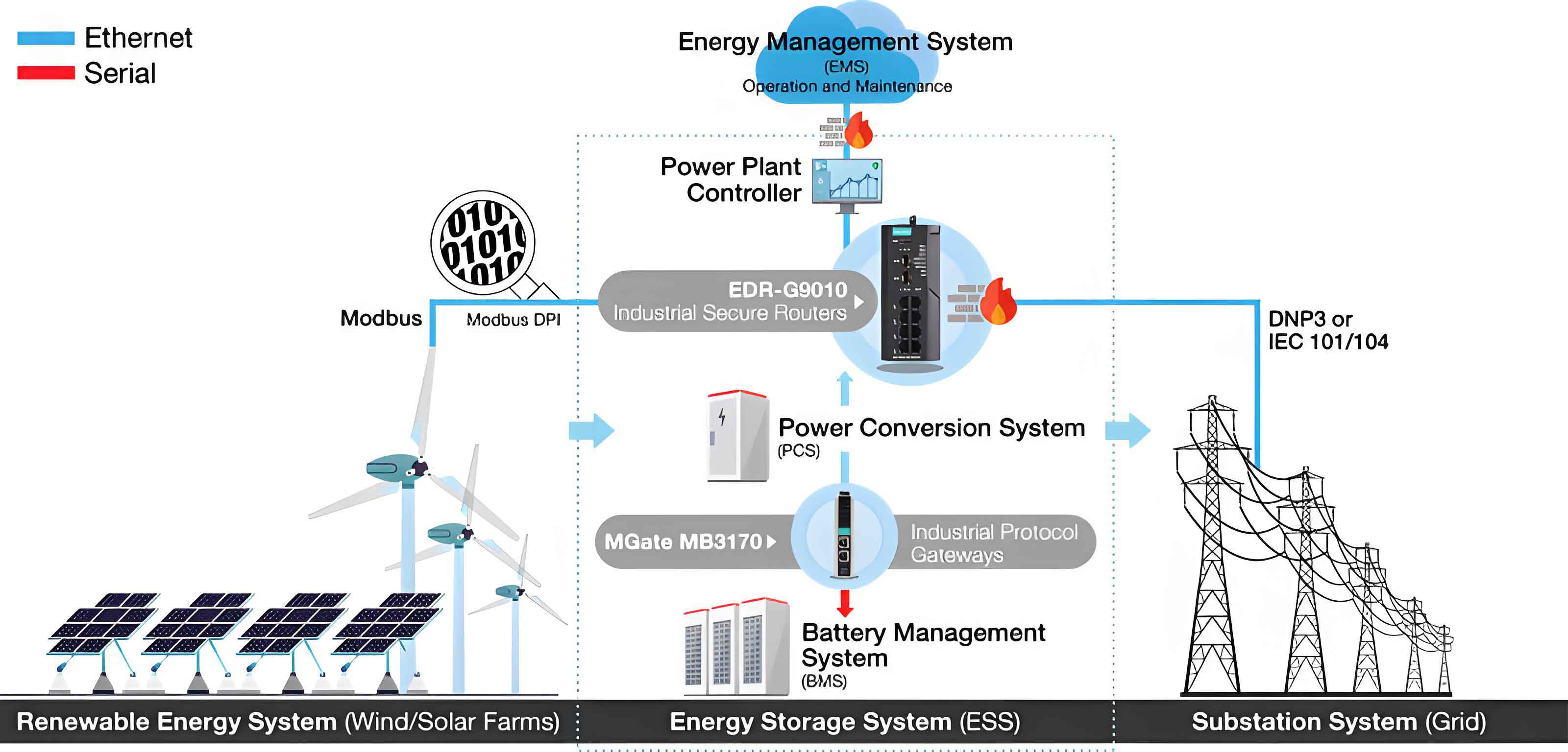
1. ESS Cycle Life Modeling
The cycle life of an energy storage system is quantified using depth-of-discharge (DoD)-dependent degradation. The equivalent daily cycles under 100% DoD are calculated as:
$$ l_{100,j,day} = \sum_{t=1}^{T} \left[ l_{100,j,t} – (1 – g_{j,t}) l_{100,j,t-1} \right] $$
where \( g_{j,t} \) represents charging state transitions, and \( l_{100,j,t} \) is derived from the polynomial fitting:
$$ l = -2083d_j^3 + 8750d_j^2 – 13170d_j + 11200 $$
2. Two-Stage Distributionally Robust Optimization
The optimization model considers PV uncertainty through adjustable Kullback-Leibler (KL) divergence-constrained ambiguity sets:
$$ \Omega_{\varsigma} = \left\{ \tilde{\varsigma} \mid \Phi_{\text{ADKL}}(\tilde{\varsigma}, \varsigma) \geq \sigma \right\} $$
Objective function maximizes system profit:
$$ \max_{x \in X} \min_{\rho_n \in \Omega_\varsigma} \sum_{n=1}^N \rho_n \max_{y_n \in Y} \left[ c_h \sum_{t \in T_h} P_{L,t} + c_v \sum_{t \in T_v} P_{L,t} + c_f \sum_{t \in T_f} P_{L,t} – c_g \sum_{t=1}^T P_{G,t} – f_{\text{main}} + f_p \right] $$
3. Key Constraints
ESS Operational Limits:
$$ \begin{cases}
E_{\text{ESS},j,t+1} = E_{\text{ESS},j,t}(1-\delta_s) + \left( \eta P_{\text{ch},j,t} – \dfrac{P_{\text{di},j,t}}{\eta} \right) \Delta t \\
\alpha_s E_{\text{ESS},j,N} \leq E_{\text{ESS},j,t} \leq E_{\text{ESS},j,N} \\
P_{\text{ch},j,t} \leq y_{\text{ch},j,t} P_{\text{ch},j,\max} \\
P_{\text{di},j,t} \leq y_{\text{di},j,t} P_{\text{di},j,\max}
\end{cases} $$
Demand Response:
$$ \begin{bmatrix}
\Delta P_{L,h} \\
\Delta P_{L,v} \\
\Delta P_{L,f}
\end{bmatrix} =
\begin{bmatrix}
P_{L,h,0} & 0 & 0 \\
0 & P_{L,v,0} & 0 \\
0 & 0 & P_{L,f,0}
\end{bmatrix}
\mathbf{D}
\begin{bmatrix}
\Delta c_h/c_{h,0} \\
\Delta c_v/c_{v,0} \\
\Delta c_f/c_{f,0}
\end{bmatrix} $$
4. Convexification Techniques
Non-convex constraints are addressed through:
- Big-M method for binary-continuous products
- McCormick envelopes for bilinear terms
- Second-order cone relaxation for AC power flow
5. Benefit Allocation via Improved Shapley Value
The modified Shapley value method incorporates PV utilization rates:
$$ \omega_r = \frac{\theta_r}{\sum \theta_r}, \quad W_r = M_r + \frac{1}{n}(1 – \omega_r)C(S) $$
where \( \theta_r \) represents PV utilization when ESS \( r \) operates independently.
6. Case Study Results
| Scenario | DR | ESS Aging | Revenue (M¥/day) | ESS Cost (k¥/day) |
|---|---|---|---|---|
| 1 | No | No | 206.53 | 2.00 |
| 4 | Yes | Yes | 148.42 | 3.90 |
| 7 | Yes | Yes | 140.16 | 3.62 |
Key findings:
- DR reduces peak-valley difference by 29.16% but increases grid purchase cost by 0.54-1.90%
- Considering ESS cycle life improves total benefits by 1-2% despite higher maintenance costs
- Distributionally robust optimization achieves 3-5% higher benefits than traditional robust methods
7. ESS Benefit Allocation
| ESS | Shapley Value (¥) | Improved Method (¥) | Δ (%) |
|---|---|---|---|
| 1 | 7,488 | 8,156 | +8.93 |
| 3 | 18,576 | 21,886 | +17.82 |
The improved Shapley method effectively redistributes benefits based on PV utilization contributions, enhancing fairness in multi-ESS systems.
8. Conclusion
This work demonstrates that incorporating energy storage system cycle life models and distributed robust optimization significantly improves operational efficiency in flexible distribution networks. The proposed benefit allocation strategy promotes fair participation of multiple ESS units in peak-shaving markets, facilitating large-scale energy storage system deployment.