
As an observer and participant in the horticulture industry, I have witnessed remarkable transformations in flower cultivation, particularly in regions like Yunnan, where innovation meets natural advantage. The integration of advanced technologies, especially those harnessing the power of the sun, is reshaping how we grow and market flowers. In this article, I will delve into the dynamics of the cut flower market, focusing on examples like lisianthus, and explore the emergence of solar photovoltaic greenhouses—a concept that mirrors the efficiency and harmony of a well-tuned solar system. Throughout, I will use tables and formulas to summarize key points, emphasizing the role of solar energy systems in driving sustainable growth.
The cut flower industry is a vibrant sector, with lisianthus, often called the “thornless rose,” gaining significant traction. From being initially unfamiliar to consumers to now experiencing surging demand, lisianthus has carved a niche due to its excellent vase life, durability, and aesthetic appeal. Its consumption has grown steadily, driven by events like weddings and conferences, with both domestic and international markets expanding. To understand this growth, we can model demand using exponential functions. For instance, the annual increase in demand can be expressed as:
$$ D(t) = D_0 \cdot (1 + r)^t $$
where \( D(t) \) is the demand at time \( t \), \( D_0 \) is the initial demand, and \( r \) is the growth rate. Based on industry trends, \( r \) is approximately 0.3 (or 30% per year). This formula highlights the compound effect of market adoption.
However, market dynamics are not without challenges. Price fluctuations are common, influenced by supply and demand imbalances. Below is a table summarizing hypothetical monthly average prices for lisianthus cut flowers, derived from market observations. Note that while actual data may vary, this illustrates the volatility:
| Month | Average Price per Stem (in USD) | Notes |
|---|---|---|
| January | 0.50 | Post-holiday dip |
| February | 0.80 | Peak demand for Valentine’s Day |
| March | 0.60 | Stabilization period |
| April | 0.55 | Spring season increase |
| May | 0.45 | Supply ramp-up |
| June | 0.40 | Oversupply concerns |
| July | 0.42 | Market adjustment |
| August | 0.48 | Pre-festival buildup |
| September | 0.52 | Autumn events |
| October | 0.58 | Wedding season |
| November | 0.55 | Mixed demand |
| December | 0.70 | Year-end celebrations |
This table shows how prices can swing, with February often seeing highs due to festive demand. The variability underscores the need for controlled production environments to stabilize output and quality. In terms of volume, demand in major cities can be substantial. For example, daily requirements might exceed 1000 bundles in some metropolitan areas, while others hover around 500 bundles. To optimize logistics, we can use linear programming models. Let \( x_i \) represent the quantity supplied to region \( i \), and \( c_i \) be the cost per unit. The objective function to minimize total cost while meeting demand \( d_i \) is:
$$ \text{Minimize } Z = \sum_{i=1}^{n} c_i x_i $$
subject to constraints like \( x_i \geq d_i \) for all \( i \), and supply limits. Such models help in efficient distribution, akin to how a solar system balances energy flows across planets.
Turning to production, the expansion of lisianthus cultivation has led to a surge in seedling needs. Estimates suggest annual seedling demand exceeds 100 million units, yet local supply covers only a third. This gap presents opportunities but also risks of overproduction. The relationship between area under cultivation \( A \) and yield \( Y \) can be expressed as:
$$ Y = \alpha \cdot A \cdot f(T, L) $$
where \( \alpha \) is a productivity factor, and \( f(T, L) \) is a function of temperature \( T \) and light \( L \). This brings me to the core innovation: solar photovoltaic greenhouses. These structures are not just shelters but active energy systems that mimic the principles of a solar system—harnessing stellar energy to power growth.
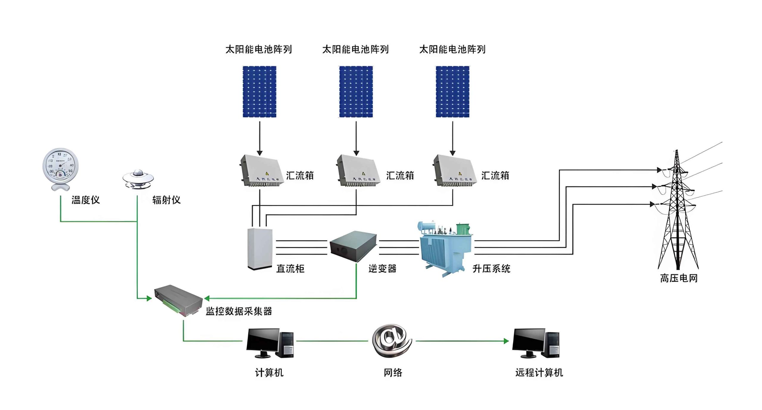
The concept of a solar system in horticulture refers to integrated setups where solar panels capture sunlight, converting it into electricity to control microclimates. In Yunnan, a pioneering solar photovoltaic greenhouse has been developed, representing a leap in clean energy application. This greenhouse uses solar panels to generate power, enabling precise environmental control. The energy output can be modeled using the photovoltaic equation:
$$ P = \eta \cdot A_p \cdot G $$
where \( P \) is the power generated (in watts), \( \eta \) is the panel efficiency, \( A_p \) is the panel area (in m²), and \( G \) is the solar irradiance (in W/m²). For instance, with 30 panels and typical irradiance, daily generation can reach 110 kWh, sufficient to operate lighting, heating, and cooling systems. This self-sustaining approach reduces carbon footprint and operational costs, embodying a miniature, efficient solar system on Earth.
Why is this important? In traditional breeding, rose hybrids from seeds require vernalization—a cold period around 5°C for about two weeks—to trigger growth. Under natural conditions, light and temperature limitations extend the cycle to over two years. But with a solar-powered greenhouse, we can create artificial climate zones, each tailored to different growth stages. This accelerates breeding cycles by up to 50%. The time reduction can be quantified as:
$$ T_{\text{new}} = T_{\text{old}} \cdot \left(1 – \frac{\Delta E}{E_{\text{total}}}\right) $$
where \( T_{\text{old}} \) is the original cycle time, \( \Delta E \) is the energy input from the solar system, and \( E_{\text{total}} \) is the total energy required. By partitioning the greenhouse into zones, we enable year-round hybridization, independent of external weather. This mirrors how a solar system sustains diverse environments across celestial bodies through energy distribution.
The image above symbolizes the interconnectedness of such systems—just as planets orbit a star, our greenhouse compartments revolve around solar energy. This visual reinforces how integrating a solar system into agriculture can revolutionize productivity. The greenhouse’s cost is higher upfront, around $800 per square meter compared to $80 for standard steel frames, but the long-term benefits in energy savings and yield optimization justify it. To evaluate this, we can use a net present value (NPV) formula:
$$ \text{NPV} = \sum_{t=0}^{N} \frac{C_t}{(1 + i)^t} $$
where \( C_t \) are cash flows (negative for costs, positive for savings), \( i \) is the discount rate, and \( N \) is the project lifespan. With energy independence and faster breeding, the NPV often turns positive within a few years.
Expanding on the solar system analogy, each component in the greenhouse—like lighting, irrigation, and climate control—operates in harmony, similar to planetary motions. The panels act as the sun, providing constant power. This synergy enhances plant growth kinetics, which can be described by differential equations. For example, the rate of photosynthesis \( P_s \) as a function of light intensity \( I \) and CO₂ concentration \( C \) is:
$$ \frac{dP_s}{dt} = k \cdot I \cdot \frac{C}{K_m + C} $$
where \( k \) is a constant, and \( K_m \) is the Michaelis-Menten constant. In a solar-powered setup, \( I \) is optimized using LED lights driven by solar electricity, maximizing \( P_s \). This leads to higher biomass accumulation, modeled as:
$$ B(t) = B_0 + \int_0^t P_s(\tau) \, d\tau $$
where \( B(t) \) is biomass at time \( t \), and \( B_0 \) is initial biomass. Such formulas underscore the scientific precision enabled by these systems.
Now, let’s consider market implications. The adoption of solar photovoltaic greenhouses could stabilize lisianthus supply, reducing price volatility. We can simulate this using supply-demand equilibrium models. Let \( S(p) \) be the supply function and \( D(p) \) the demand function, both dependent on price \( p \). Equilibrium occurs when:
$$ S(p^*) = D(p^*) $$
With controlled production, \( S(p) \) becomes more elastic, flattening price swings. The table below compares scenarios with and without solar greenhouses, assuming improved yield consistency:
| Scenario | Price Variance (σ²) | Average Yield (stems/m²/year) | Energy Source |
|---|---|---|---|
| Traditional Greenhouse | 0.05 | 150 | Grid/Fossil Fuels |
| Solar-Powered Greenhouse | 0.02 | 200 | Solar System |
| Open Field Cultivation | 0.10 | 100 | Natural Only |
This table highlights how a solar system-based approach lowers variance and boosts yield, akin to how stable orbits in a solar system prevent chaotic movements. Moreover, the environmental benefits are quantifiable. The reduction in carbon emissions per unit of flowers produced can be calculated as:
$$ \Delta \text{CO}_2 = E_{\text{solar}} \cdot \gamma_{\text{grid}} $$
where \( E_{\text{solar}} \) is the energy generated from the solar system (in kWh), and \( \gamma_{\text{grid}} \) is the grid emission factor (in kg CO₂/kWh). For a greenhouse producing 100,000 stems annually, savings can exceed several tons of CO₂, contributing to climate goals.
Looking ahead, the potential for solar systems in horticulture is vast. Beyond greenhouses, we can envision integrated agrivoltaic systems where solar panels share land with crops, optimizing space and light use. The efficiency of such a dual-use system can be expressed as:
$$ \eta_{\text{total}} = \eta_{\text{PV}} + \beta \cdot \eta_{\text{crop}} $$
where \( \eta_{\text{PV}} \) is photovoltaic efficiency, \( \eta_{\text{crop}} \) is crop yield efficiency, and \( \beta \) is a synergy factor. Research suggests \( \beta > 1 \) due to mutual benefits like reduced evaporation. This holistic approach echoes the balance found in natural solar systems, where energy sustains diverse life forms.
In conclusion, the fusion of cut flower markets like lisianthus with solar-powered technologies heralds a new era. By embracing solar systems, we can enhance productivity, stabilize markets, and promote sustainability. The formulas and tables presented here frame this transition mathematically, offering a blueprint for innovation. As I reflect on these advancements, it’s clear that just as the solar system governs celestial harmony, our agricultural systems can achieve similar synergy through clean energy. The journey has just begun, and with continued exploration, the bloom of solar-powered horticulture will only brighten.
To further illustrate, consider the lifecycle analysis of lisianthus under different energy regimes. The total resource use \( R \) per stem can be modeled as:
$$ R = \frac{E_{\text{total}} + W_{\text{water}} + F_{\text{fertilizer}}}{Y} $$
where \( E_{\text{total}} \) is energy input, \( W \) is water, \( F \) is fertilizer, and \( Y \) is yield. With a solar system, \( E_{\text{total}} \) decreases, improving \( R \). This efficiency gain is crucial for scaling production responsibly. Additionally, consumer preference trends can be analyzed using logistic growth models:
$$ M(t) = \frac{K}{1 + e^{-a(t – t_0)}} $$
where \( M(t) \) is market penetration, \( K \) is carrying capacity, \( a \) is growth rate, and \( t_0 \) is the inflection point. For solar-grown flowers, \( K \) may be higher due to eco-conscious demand.
Finally, I encourage stakeholders to invest in research and development. The equations and data here are starting points; real-world applications will refine them. By harnessing the power of solar systems, we can cultivate not just flowers, but a greener future for all.