
1. Equivalent circuit of solar cells
Solar cells can be represented by different equivalent circuits, but the most commonly used is the single diode equivalent circuit, as shown in Figure 1.
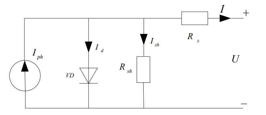
In the figure, we consider the current generated by the solar cell as a constant current source Iph, with a diode connected in parallel and a leakage current of Id, known as dark current. Dark current is the current flowing through the P-N junction under external voltage in the absence of light. The dark current Id can be expressed as:
Among them,
I0- Reverse saturation current of the diode, A;
U – output voltage, V;
Q – charge quantity, C;
T – temperature, ℃;
K – Boltzmann constant.
N – The ideal factor of the diode, with a value between 1 and 2, often taken as around 1.3.
The expression for the output current I can be derived as follows:
In practical applications, in order to simplify calculations, the influence of parallel resistors is usually not considered, and it is considered that parallel resistors are infinitely large. So, the simplified output current expression is:
2. Output characteristics of solar cells
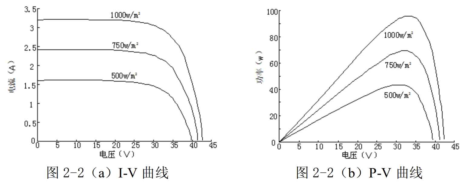
From the equivalent circuit and output expression above, it can be seen that the output characteristics of solar cells are related to external temperature and light intensity to a certain extent. Assuming an ambient temperature of 25 ℃ and light intensity of 500 w/m ^ 2750 w/m ^ 2 and 1000 w/m ^ 2, the P-V and I-V curves of the solar cell are shown in Figure 2. With the increase of light intensity, the voltage does not change much, but the output current has a significant change, and the output power also increases accordingly. From this, it can be seen that light intensity is an important factor affecting the output power.
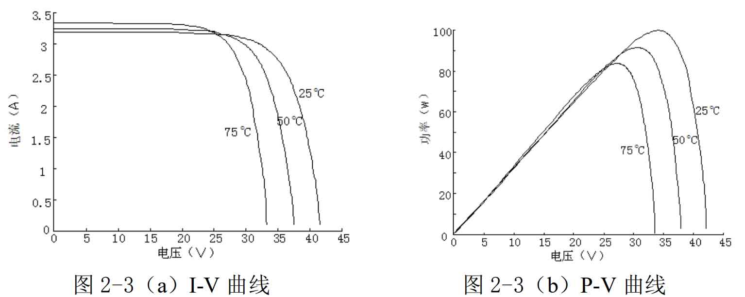
When the light intensity is 1000 w/m ^ 2 and does not change, the temperature is set to 25 ℃, 50 ℃, and 75 ℃. The P-V and I-V curves of the solar cell are shown in Figure 3. As the temperature increases, the output current of the solar cell slightly increases, but the voltage gradually decreases, and the output power changes greatly and gradually decreases. It can be seen that external temperature is also another important factor affecting output power.
Because solar cells are non-linear power sources, differences in external temperature and light intensity can lead to changes in output power. But at a certain temperature and light intensity, there will be a maximum output power point, which is commonly referred to as the maximum power point. Therefore, in practical systems, we must detect solar cells and control and sample them to ensure that they always work near the maximum power point, in order to achieve maximum power point tracking.
3. Maximum power point tracking technology
One of the main drawbacks of photovoltaic power generation systems is that the photoelectric conversion efficiency is too low. Generally, polycrystalline silicon cells account for 12% to 14%, while monocrystalline silicon cells account for 14% to 18%. If we consider the conversion efficiency of solar inverters again, the comprehensive efficiency of photovoltaic power generation systems is only about 10%. In order to maximize the utilization of solar energy, firstly, to improve the conversion efficiency of photovoltaic arrays; The second is to adopt effective methods in the structure or control of solar inverters to adjust the working point of the photovoltaic array in real time, so that it always works near the maximum power point. This adjustment process is called maximum power point tracking.
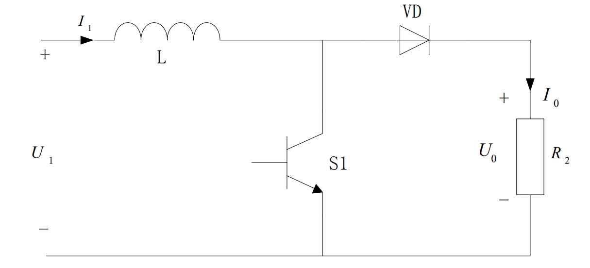
In photovoltaic power generation systems, the direct current obtained from the output voltage of the solar cell through the Boost boost circuit is usually used as the input of the solar inverter. To achieve maximum power point tracking during the boosting process. Let the output voltage of the solar cell be U1, the output current be I1, the duty cycle be D, and R2 be the load. The topology of the Boost boost circuit is shown in Figure 4:
According to the formula:
At this point, we will equivalent the DC/DC converter and load to a variable resistor Req, which is related to the duty cycle D and load R2. Let P be the output power of the solar cell.
By combining the formula to eliminate Req, it can be concluded that:
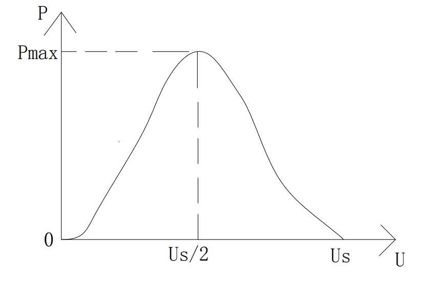
When U1=Us/2, there is maximum power output:
The P-U curve of the solar cell is shown in Figure 5. When U1=Us/2, i.e. R1=Req, the output power is at its maximum. So, while keeping R2 constant, we can achieve maximum power point tracking by changing the duty cycle D to make R1=Req.
According to circuit theory, when the output impedance of a solar cell is equal to the load impedance, the solar cell can output the maximum power. From this, it can be seen that the maximum power point tracking process is actually the process of matching the output impedance with the load impedance. Under uniform illumination, the output power of solar cells follows a single peak curve, and the properties of the curve’s extreme points indicate that:
When the duty cycle is 1, the load resistance R2=R, and when the duty cycle is 0, R 2=∞.
The input-output relationship of the switching tube is:
Substituting the formula yields:
At maximum power point, based on the characteristics of the solar cell:
From this, it can be concluded that:
From this, the change in output power can be achieved by changing the duty cycle, that is, if the duty cycle at the maximum power point is found, the maximum power point can be found.
There are currently many methods used for MPPT, including constant voltage method, incremental conductance method, disturbance observation method, and intelligent algorithm based MPPT method. This section conducts research and analysis on the commonly used incremental conductivity method.
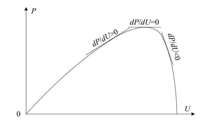
The incremental conductance method is a method of tracking the maximum power point by comparing the instantaneous impedance and impedance change of a photovoltaic array. According to the P-V curve, at the maximum power point, the power derivative with respect to voltage is zero. The power expression of the photovoltaic array is P=UI, and taking the derivative of U at both ends yields dP/dU=1+U dI/dU=0, that is, dI/dU=- I/U.
The working principle diagram of the incremental conductivity method is shown in Figure 6:
When dP/dU=0, the solar cell operates at its maximum power point. The relationship equation at the maximum power point is:
In practice Δ I/ Δ U approximates dI/dU to obtain the maximum power point tracking criterion:
(1) Δ I/ Δ U>- I/U working point is on the left side of the maximum power point.
(2) Δ I/ Δ U=- I/U working point is the maximum power point.
(3) Δ I/ Δ U<- I/U working point is on the right side of the maximum power point.
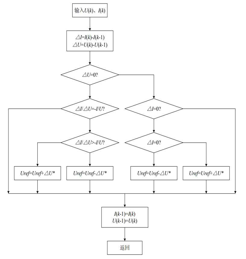
The flowchart of the conductivity increment algorithm is shown in Figures 7, where the voltage adjustment step size is Δ U *, Uref For the next working point voltage.
In order to study the maximum power point tracking of Boost circuits more simply and intuitively, we equivalent the inverter and load in the later stage to a resistor, and package the control module of maximum power point tracking into a submodule. The simulation model based on the incremental conductivity method is shown in Figure 8: we set the external temperature to 25 ℃, and we use a step function to simulate the changes in light intensity S. We observe the changes in output voltage and current, as well as the changes in power, through an oscilloscope.
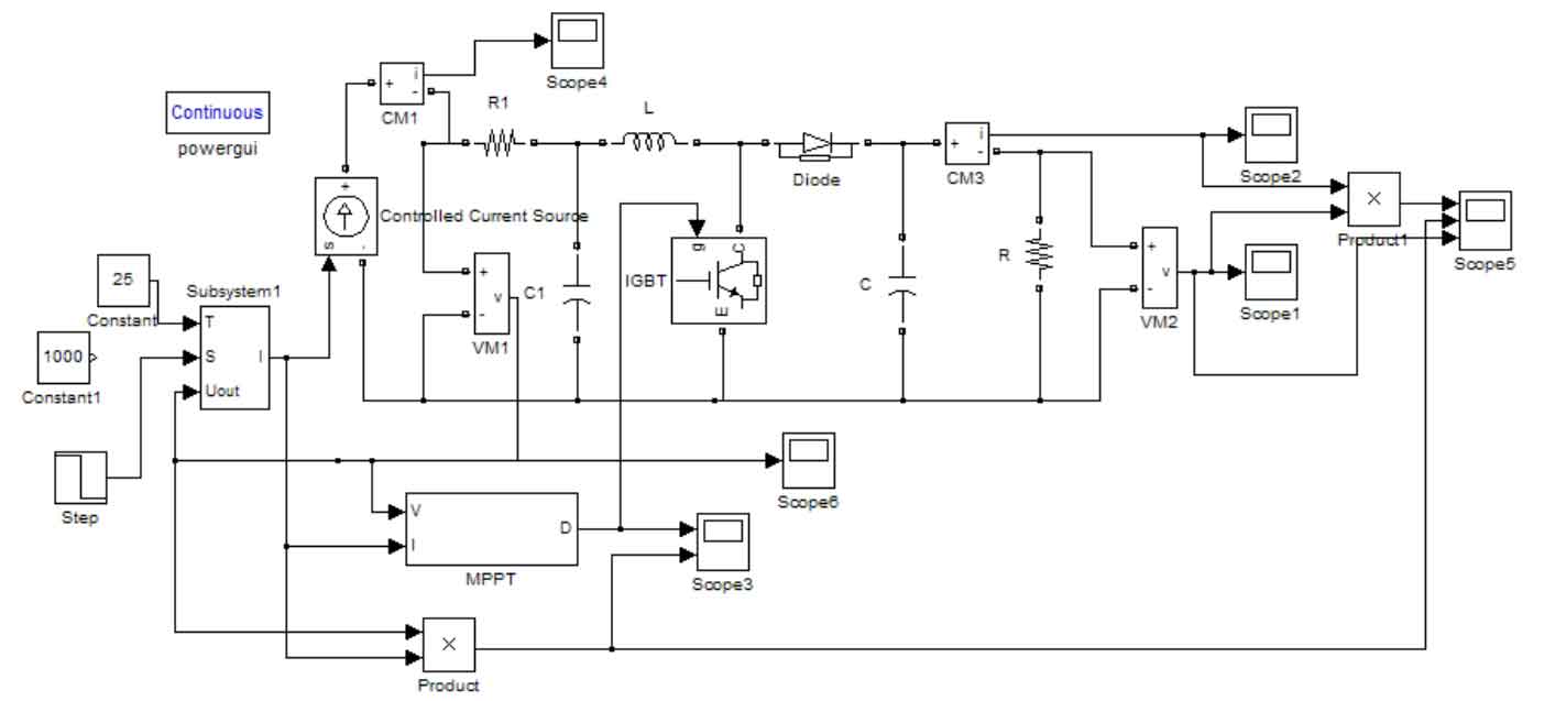
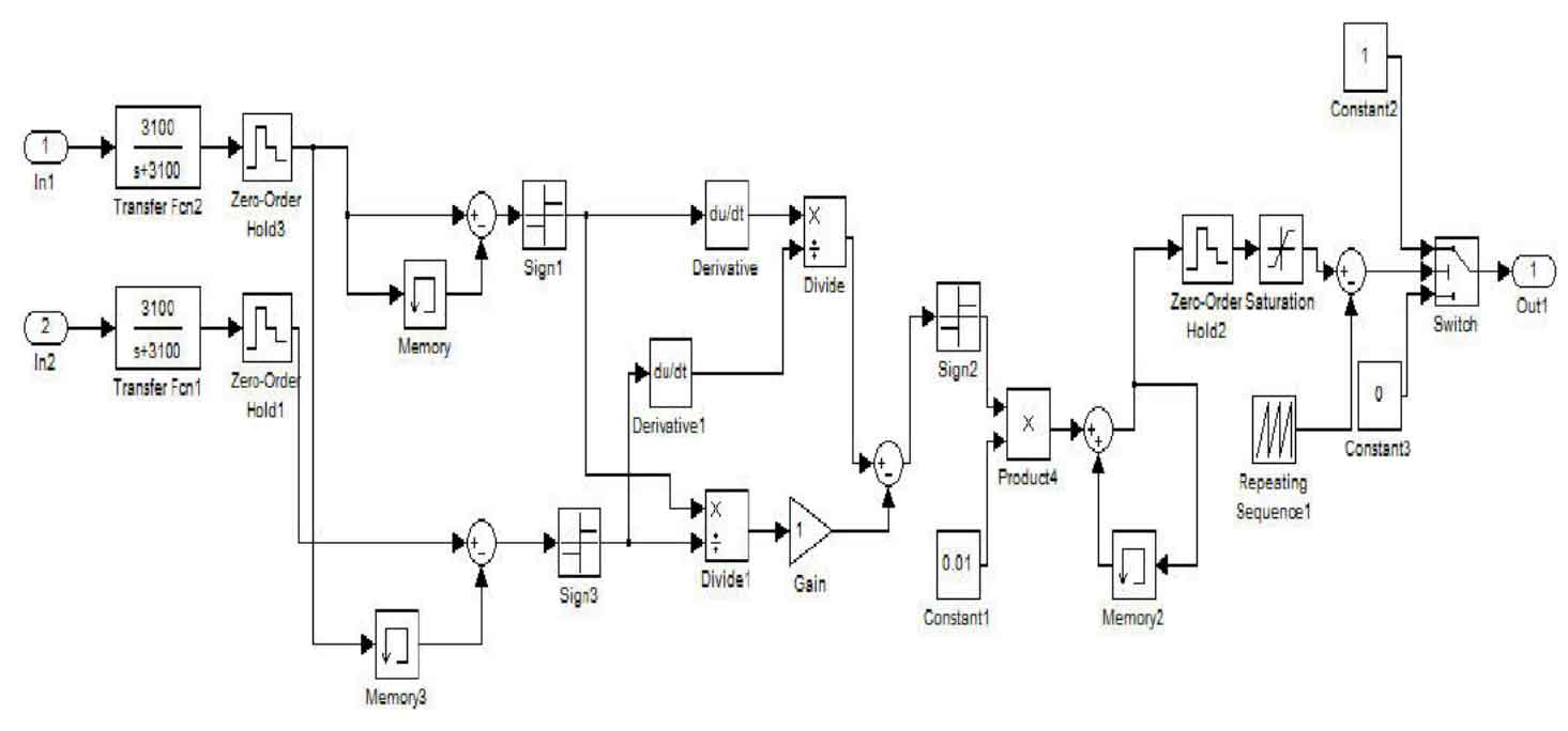
The model of the control algorithm for maximum power point tracking using the incremental conductance method is shown in Figure 9. Firstly, we delay the collected output voltage and current and subtract them from the original values to obtain the corresponding values Δ U and Δ I. After taking the derivative separately, the disturbance direction of the current duty cycle is obtained through the symbol module. Then multiply by 0.01, Δ When D is the positive disturbance direction, take 0.01, otherwise take -0.01. After the delay phase, the duty cycle D (n)=D (n-1) is obtained+ Δ D. After comparing with the carrier wave, obtain the modulation wave and control the on/off of the switching tube.
After simulation, the obtained graph is shown in Figure 10: after a period of time, the solar cell tends to operate in a stable state, and the output power of the solar cell is close to stability. After Boost boost, it also tends to stabilize and operates near the maximum power point.
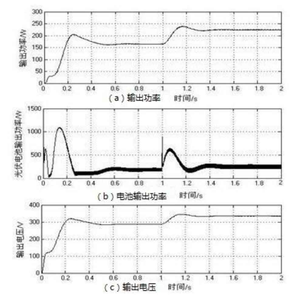
At 1 second, the light intensity changes, and the output voltage and power of the solar cell also change. Through tracking the maximum power point by the system, the output power of the system also changes and always works near the maximum power point. It can be seen that this method can quickly track the maximum power point and the tracking waveform is relatively stable. We can change it by Δ The value of D is used to further improve the output waveform curve.
Although the incremental conductance method can achieve tracking of the maximum power point, it requires high accuracy in the detection system and the calculation process is relatively complex, so it is greatly limited in certain situations. In the current era of intelligence, it is urgent to seek another more effective method.