
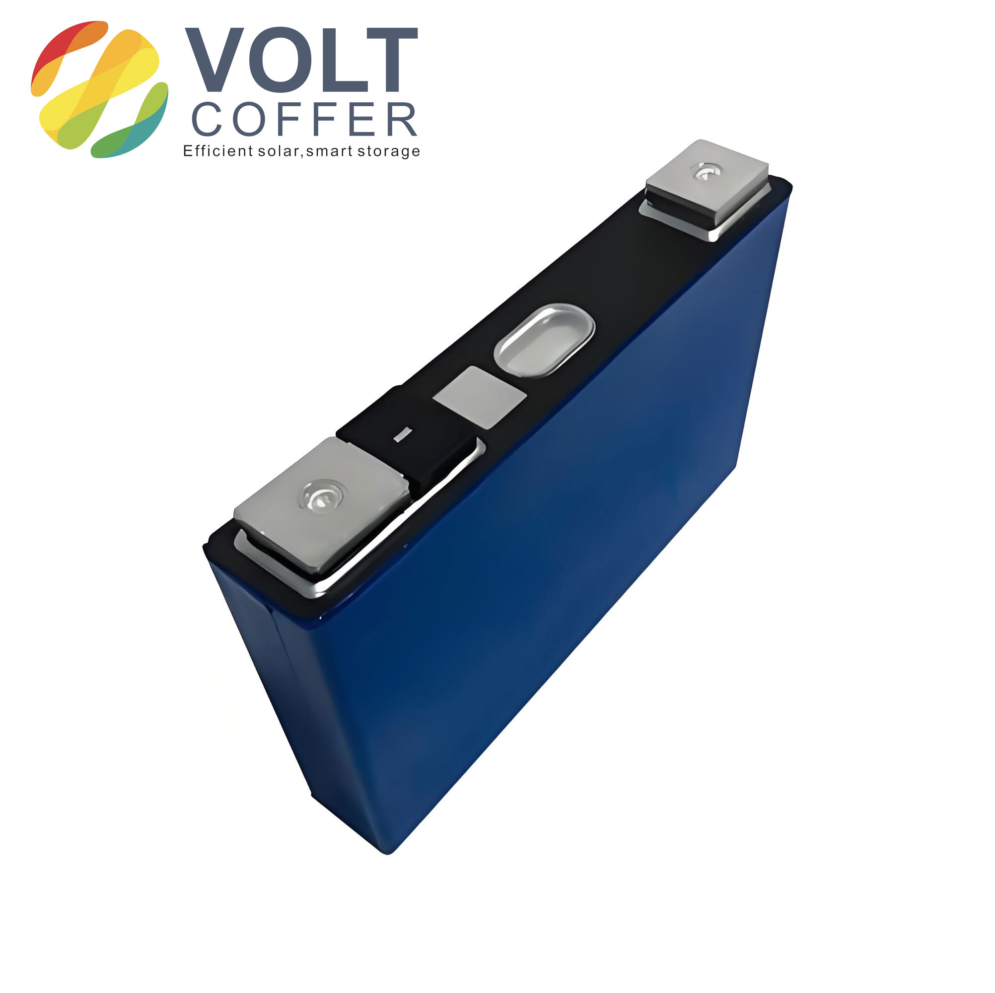
I treat the state of health of a lithium ion battery as a proactive state-awareness variable for low-voltage TN-C-S distribution systems rather than as a direct leakage or trip criterion. In my view, the degradation of a lithium ion battery is one of the earliest measurable indicators of reduced operating margin in an energy storage branch. As a lithium ion battery ages, its internal resistance increases, its available capacity decreases, its thermal stress accumulates, and its insulation-related performance may decline under coupled electrical and environmental stresses. These changes do not map one-to-one to residual current, zero-sequence voltage offset, or protective tripping, but they provide a useful pre-fault indication that can complement conventional residual-current detection.
I therefore construct a lithium ion battery SOH estimation framework based on a RIME-optimized temporal convolutional network and Transformer, denoted RIME-TCN-Transformer. The purpose is not to replace residual-current protection or zero-sequence monitoring. Instead, I use high-precision lithium ion battery SOH estimation as an upstream aging-state sensing layer that can be integrated into an intelligent monitoring terminal of a TN-C-S distribution area. The output can be combined with residual current, zero-sequence voltage, and protection actions to form a layered safety architecture: health-state awareness, electrical-safety detection, and protective action.
Motivation and Safety Context
I begin with the observation that low-voltage distribution networks are the final electrical link to end users, and their safety performance directly affects electric shock risk and electrical fire risk. In a TN-C-S system, the front-end PEN conductor is separated at the user entry into a neutral conductor and a protective earth conductor. The protective earth conductor is repeatedly grounded and then laid independently from the neutral conductor. This arrangement supplies a protective grounding path for power conversion systems, battery management systems, and other core equipment in a lithium ion battery energy storage installation. However, the shared PEN section creates distinctive risks, including zero-sequence voltage offset, PEN breakage that can energize enclosures, and common-mode interference transfer.
When a lithium ion battery energy storage branch is connected to a TN-C-S low-voltage distribution system, battery capacity fade, internal resistance rise, and thermal stress accumulation reduce the operating margin of the storage branch. System-level insulation degradation is also influenced by electrical connections, environment, and equipment integration. Conventional residual-current devices act according to direct safety quantities such as residual current. A lithium ion battery SOH value itself cannot directly represent a leakage fault. I therefore treat SOH as an aging-state prior and use it together with zero-sequence voltage, residual current, and protection actions to enrich the state-awareness information available to TN-C-S safety protection.
From an electrochemical perspective, solid electrolyte interphase growth, loss of lithium inventory, and electrolyte side reactions cause capacity fade and internal resistance rise. These processes can also intensify voltage fluctuation and thermal stress during charge and discharge. Nevertheless, the relationship between lithium ion battery SOH and system insulation, residual current, and protection tripping is not one-to-one. It is also affected by connection state, ambient temperature, power conversion system operating mode, and grounding conditions. I therefore position SOH as a pre-fault aging-state sensing quantity, not as a direct leakage or trip criterion. The mapping from SOH to safety risk still requires calibration using synchronized data from the power conversion system, the battery management system, and the distribution side.
Data Sources and SOH Definition
To evaluate whether my method can estimate lithium ion battery SOH across different material systems, temperatures, and rates, I use two offline battery datasets. The first dataset is a public aging dataset of commercial 18650 lithium ion battery cells with a nickel-cobalt-aluminum oxide positive electrode and a graphite negative electrode. The rated capacity is 3.5 Ah, and the rated voltage is 4.2 V. I use two cells, labeled NCA-1 and NCA-2, for SOH estimation. The second dataset is obtained from laboratory cycle aging tests. Twelve lithium iron phosphate lithium ion battery cells are divided into four groups. Cells LFP-1 through LFP-3 form the first group, LFP-4 through LFP-6 form the second group, LFP-7 through LFP-9 form the third group, and LFP-10 through LFP-12 form the fourth group. The tests are conducted at 25 degrees Celsius. All cells are charged at 5 C. The discharge rates are 5 C, 10 C, 15 C, and 20 C for the four groups, respectively. I select LFP-1 and LFP-4 for detailed SOH estimation. The conditions are summarized in Table 1.
| Cell label | Chemistry family | Temperature | Charge rate | Discharge rate | Rated capacity | Nominal voltage |
|---|---|---|---|---|---|---|
| NCA-1 | Nickel-cobalt-aluminum oxide / graphite | 25 degrees Celsius | 0.5 C | 0.5 C | 3.5 Ah | 4.2 V |
| NCA-2 | Nickel-cobalt-aluminum oxide / graphite | 45 degrees Celsius | 0.5 C | 0.5 C | 3.5 Ah | 4.2 V |
| LFP-1 | Lithium iron phosphate | 25 degrees Celsius | 5 C | 5 C | Laboratory rated capacity | Laboratory nominal voltage |
| LFP-4 | Lithium iron phosphate | 25 degrees Celsius | 5 C | 10 C | Laboratory rated capacity | Laboratory nominal voltage |
I define the state of health of a lithium ion battery as the ratio of the current available maximum capacity to the rated capacity:
$$ SOH = \frac{Q_{act}}{Q_0} $$
Here, \(Q_{act}\) is the current available maximum capacity, and \(Q_0\) is the rated capacity. In my experiments, I use discharge capacity as a positive proportional representation of SOH. Because a positive proportional transformation does not change sample ranks, I can use complete-cycle samples for rank-based correlation analysis.
Health Feature Extraction
Raw charge and discharge data of a lithium ion battery contain rich aging information, but they are high-dimensional and redundant. Direct use as model input increases computational complexity and slows convergence. I therefore extract health features that are physically meaningful, statistically correlated with SOH, and measurable under field conditions. I consider three sources: time-domain behavior, incremental capacity, and voltage relaxation.
During constant-current charging, polarization voltage increases as the lithium ion battery ages. The terminal voltage reaches the cutoff voltage more quickly, so the constant-current charging time decreases with cycling. During constant-voltage charging, increased internal resistance and reduced diffusion rate prolong the time required to complete the constant-voltage stage. I initially considered both constant-current charging time and constant-voltage charging time as health features.
Charge and discharge plateau durations also reflect lithium ion battery aging. Voltage plateaus and slow-change regions are closely related to lithium insertion and extraction reactions and phase evolution. As loss of lithium inventory and loss of active material accumulate, the effective reaction charge within a given voltage interval decreases. At the same time, increased internal resistance and polarization cause the charge and discharge processes to reach cutoff voltage earlier, shortening the effective plateau duration. For example, in one NCA cell at 25 degrees Celsius over 208 complete cycles, when SOH decreases from 93.40 percent to 72.82 percent, the charge plateau duration decreases from 3668.43 s to 3028.22 s, a reduction of 17.45 percent. The discharge plateau duration decreases from 2364.83 s to 1811.36 s, a reduction of 23.40 percent. Linear regression indicates that for every one percentage point decrease in SOH, the charge and discharge plateau durations shorten by 25.82 s and 24.99 s, respectively, with coefficients of determination of 0.9817 and 0.9826. A second NCA cell at 45 degrees Celsius shows the same trend, with charge and discharge plateau durations decreasing by 15.23 percent and 15.53 percent. This confirms that plateau shortening with SOH decay is consistent across temperature conditions, although the rate differs.
The incremental capacity curve is obtained by differentiating capacity with respect to terminal voltage:
$$ IC = \frac{dQ}{dV} \approx \frac{Q_k – Q_{k-N}}{V_k – V_{k-N}} $$
Here, \(Q_k\) and \(V_k\) are the capacity and terminal voltage at sampling point \(k\), and \(N\) is the difference interval. The differentiation amplifies voltage and capacity sampling noise. I apply Gaussian smoothing to voltage and capacity measurement sequences before calculating \(dQ/dV\). I extract the incremental capacity peak and the voltage corresponding to the incremental capacity peak as candidate health features.
Both datasets include rest periods after charge and discharge. I specifically extract the voltage rebound during the discharge relaxation stage as a candidate health feature. Compared with dynamic conditions, the relaxation stage can characterize internal dynamics with relatively small load-current disturbance. It can serve as a useful supplement to dynamic features. However, the voltage rebound during discharge relaxation is a combined result of ohmic polarization, concentration polarization, and activation polarization recovery. Its evolution is sensitive to discharge depth, discharge rate, rest duration, and ambient temperature. It also depends on a relatively clear and complete rest window. In actual distribution-area energy storage operation, charge and discharge scheduling is flexible, and rest periods and durations often vary with dispatch requirements. Therefore, stable acquisition of this feature is constrained by operating conditions.
I initially extract seven candidate health factors from time-domain behavior, incremental capacity curves, and voltage relaxation. I then use the Spearman rank correlation coefficient to quantify the monotonic relationship between each candidate feature and lithium ion battery SOH. The Spearman coefficient is calculated as:
$$ \rho_s = 1 – \frac{6 \sum_{i=1}^{n} d_i^2}{n(n^2 – 1)} $$
Here, \(d_i\) is the rank difference between paired observations, and \(n\) is the number of samples. The coefficient ranges from \(-1\) to \(1\). Its absolute value indicates correlation strength, and its sign indicates direction. A value approaching \(1\) indicates a strong monotonic relationship. A positive value means the health factor increases with SOH, while a negative value means it decreases with SOH.
To reduce the risk of type I error accumulation from multiple hypothesis testing, I use the Benjamini-Hochberg method to control the false discovery rate. I use \(q < 0.05\) as the statistical significance criterion. The significance test is used to judge whether there is sufficient evidence for a statistical association between a candidate feature and SOH. It is not the only basis for feature inclusion. Final selection also considers correlation strength, redundancy among features, electrochemical aging mechanisms, and practical acquisition conditions. The candidate features and my selection decisions are summarized in Table 2.
| Feature ID | Feature description | Physical meaning | Online measurability | Selection decision |
|---|---|---|---|---|
| F1 | Constant-current charging time | Reflects polarization growth and earlier cutoff under aging | Can be extracted from battery management system voltage-current time series | Selected |
| F2 | Constant-voltage charging time | Reflects diffusion limitation and internal resistance rise | Requires voltage and current records but is affected by cutoff conditions | Not selected as primary input |
| F3 | Incremental capacity peak | Reflects reaction-region evolution and active material loss | Conditionally measurable when constant-current capacity-voltage trajectory is complete | Selected as conditional feature |
| F4 | Voltage at incremental capacity peak | Reflects peak shift and phase evolution | Sensitive to voltage resolution and smoothing | Not selected due to redundancy |
| F5 | Charge plateau duration | Reflects effective charge accepted in plateau region | Can be extracted from conventional voltage-current records | Selected |
| F6 | Discharge plateau duration | Reflects effective discharge delivered in plateau region | Can be extracted from conventional voltage-current records | Selected |
| F7 | Discharge relaxation voltage rebound | Reflects polarization recovery and internal dynamics | Depends on complete rest window and is sensitive to depth, rate, and temperature | Not selected due to operating constraints |
After Benjamini-Hochberg false discovery rate correction, all seven candidate health factors show statistically significant correlations with SOH at \(q < 0.05\). However, their correlation strength, information independence, and engineering applicability differ. Constant-current charging time, incremental capacity peak, charge plateau duration, and discharge plateau duration have Spearman correlation coefficients of 0.9966, 0.9993, 0.9932, and 0.9937, respectively. They show strong monotonic correlations and reflect lithium ion battery aging from different perspectives: charging process behavior, incremental capacity characteristics, and charge-discharge plateau evolution. They therefore have good mechanistic complementarity. I select these four features as model inputs. Table 3 summarizes the correlation and significance results.
| Feature | Spearman correlation with SOH | Adjusted q-value | Statistical significance | Role in final model |
|---|---|---|---|---|
| Constant-current charging time | 0.9966 | Less than 0.05 | Significant | Primary time-domain input |
| Incremental capacity peak | 0.9993 | Less than 0.05 | Significant | Conditional capacity-increment input |
| Charge plateau duration | 0.9932 | Less than 0.05 | Significant | Primary plateau input |
| Discharge plateau duration | 0.9937 | Less than 0.05 | Significant | Primary plateau input |
| Constant-voltage charging time | Significant but weaker | Less than 0.05 | Significant | Excluded due to weaker stability |
| Incremental capacity peak voltage | Significant | Less than 0.05 | Significant | Excluded due to redundancy |
| Discharge relaxation voltage rebound | Significant | Less than 0.05 | Significant | Excluded due to rest-window dependence |
Online Measurability and Noise Boundary of Incremental Capacity Features
Constant-current charging time and charge-discharge plateau durations can be calculated from voltage-current time series collected by a battery management system. They do not require additional dedicated sensors. However, their effective extraction still depends on the presence of a constant-current operating window of sufficient duration. In contrast, obtaining the incremental capacity peak requires a relatively continuous and complete constant-current charge capacity-voltage trajectory. It imposes higher requirements on voltage sampling resolution, sampling noise, and data continuity. I therefore define the incremental capacity peak as a conditionally measurable feature, distinct from time-domain features that can be extracted from routine operation data. When a complete constant-current charge segment is unavailable, or when data quality is insufficient for stable incremental capacity reconstruction, the incremental capacity feature can be temporarily disabled. Constant-current time and plateau durations can then serve as the main health representation.
To evaluate the sensitivity of the incremental capacity feature to measurement noise and its applicable boundary, I perform a noise perturbation experiment on 208 complete cycles. In each cycle, I add independent zero-mean Gaussian noise to the terminal voltage and charge capacity sequences during the constant-current charging stage. The noise standard deviation is determined from the root mean square value of the de-meaned original signal and the target signal-to-noise ratio. I set five signal-to-noise ratio levels: 60, 50, 40, 30, and 20 dB. Each level is independently repeated 100 times. The results are shown in Table 4.
| Target SNR (dB) | Median absolute percentage error of IC peak (%) | Median Spearman correlation with SOH | 95 percent interval of correlation | Repeats with p less than 0.05 (%) |
|---|---|---|---|---|
| 60 | 0.334 | 0.9933 | 0.9906 to 0.9949 | 100.0 |
| 50 | 1.214 | 0.9638 | 0.9520 to 0.9715 | 100.0 |
| 40 | 6.593 | 0.8500 | 0.8165 to 0.8874 | 100.0 |
| 30 | 37.943 | 0.6165 | 0.5271 to 0.6876 | 100.0 |
| 20 | 949.372 | 0.2454 | 0.1257 to 0.3920 | 96.0 |
As noise increases, the incremental capacity peak extraction error and its SOH representation ability decrease. When the signal-to-noise ratio decreases from 60 dB to 40 dB, the median absolute percentage error of the incremental capacity peak increases from 0.334 percent to 6.593 percent, and the median Spearman correlation between the incremental capacity peak and SOH decreases from 0.9933 to 0.8500. When the signal-to-noise ratio decreases further to 30 dB and 20 dB, the median correlation decreases to 0.6165 and 0.2454, respectively. At 20 dB, only 96 percent of repeated tests still satisfy \(p < 0.05\). These results indicate that at approximately 40 dB and above, the incremental capacity peak retains strong SOH ranking ability. As sampling noise increases further, feature extraction stability and health-state representation degrade. I therefore recommend dynamic selection of the incremental capacity feature according to actual sampling quality and operating completeness, rather than treating it as a fixed input without data-quality constraints.
RIME-TCN-Transformer Model
I integrate temporal convolutional network, Transformer, and RIME optimization into an SOH estimation framework for lithium ion battery health-state awareness in TN-C-S low-voltage distribution monitoring. The integration is designed under practical constraints: noticeable data disturbance, complex operating conditions, and limited computing resources at the terminal. The temporal convolutional network uses causal dilated convolution and residual structures to expand the receptive field while preserving temporal causality. It extracts local temporal features with relatively low computational overhead. It is therefore suitable for handling short-term pulse disturbance, rate mutation, and random noise in field monitoring data. It also has good parallel computing ability and edge-deployment adaptability. The Transformer uses multi-head self-attention to model dependencies at different time scales. It can capture long-term degradation trends across many cycles, compensating for the limited long-range dependency modeling of local convolution structures and enhancing representation of complex operating changes and aging trajectory drift. Because optimal hyperparameters depend on distribution-area conditions, lithium ion battery type, and data distribution, I use RIME to search key hyperparameters adaptively. This reduces manual tuning cost and improves parameter configuration efficiency in different application scenarios.
Temporal Convolutional Network
For time-series problems, temporal causality must be strictly followed. The estimate at time \(t\) can only depend on inputs at time \(t\) and earlier. A conventional convolutional neural network cannot directly handle time series without violating this constraint. The temporal convolutional network uses causal convolution to enforce this constraint. At time \(t\), the output is convolved only from inputs in the range from \(t-k\) to \(t\), where \(k\) is the convolution kernel size. A simple causal convolution has a drawback: to capture long-term time-series data, many convolutional layers or a very large kernel must be stacked, which increases computation. To solve this, the temporal convolutional network introduces dilated convolution.
For a one-dimensional sequence input \(x\) and a filter \(f:\{0,\ldots,k-1\}\rightarrow \mathbb{R}\), the dilated convolution operation \(F\) at position \(s\) is defined as:
$$ F(s) = (x *_d f)(s) = \sum_{i=0}^{k-1} f(i) \cdot x_{s – d \cdot i} $$
Here, \(d\) is the dilation factor, \(k\) is the convolution kernel size, and \(s – d \cdot i\) indicates the sampled historical time. As network depth increases, \(d\) usually grows exponentially as a power of two. This design allows the temporal convolutional network to cover a very long time span with relatively shallow network depth. To train deeper networks and improve stability, the temporal convolutional network uses residual connections. A temporal convolutional network residual block contains two dilated causal convolution layers. Each layer is followed by weight normalization and a rectified linear unit activation. The residual block output is:
$$ y = Activation(x + F(x)) $$
Here, \(x\) is the input, and \(F(x)\) is the output after a series of convolution transformations.
Transformer Module
For TN-C-S energy storage monitoring, the Transformer module captures long-term aging trends across hundreds of cycles. It complements local convolution features and improves the overall representation of complex operating fluctuations and aging trajectory changes. The Transformer structure includes an encoder and a decoder. Unlike a convolutional neural network that processes data step by step in order, the Transformer inputs the entire sequence in parallel. To allow the model to understand the temporal information of lithium ion battery data, positional encoding is required. I use sine and cosine functions for positional encoding. For an input vector of length \(L\), the positional encoding of the \(k\)-th data point is:
$$ PE(k,2i) = \sin\left(\frac{k}{n^{2i/d}}\right) $$
$$ PE(k,2i+1) = \cos\left(\frac{k}{n^{2i/d}}\right) $$
Here, \(d\) is the dimension of the input vector, and \(n\) is a user-defined scalar. The attention mechanism is the core of the Transformer. Self-attention mainly relies on three learnable linear transformation matrices: \(W_Q\), \(W_K\), and \(W_V\). The input vector is mapped by these matrices into query, key, and value matrices \(Q\), \(K\), and \(V\). After obtaining \(Q\), \(K\), and \(V\), scaled dot-product attention is calculated as:
$$ Attention(Q,K,V) = softmax\left(\frac{QK^T}{\sqrt{d_k}}\right)V $$
Here, \(QK^T\) computes the dot product to measure similarity between each query vector and key vector. The term \(\sqrt{d_k}\) is a scaling factor that prevents numerical instability caused by large dot products as vector dimension increases. The softmax function ensures that attention weights sum to one and normalizes similarity into a probability distribution. To allow the model to observe input data from different perspectives, the Transformer introduces multi-head attention:
$$ MultiHead(Q,K,V) = Concat(head_1,\ldots,head_h)W_O $$
$$ head_i = Attention(QW_i^Q, KW_i^K, VW_i^V) $$
Here, \(h\) is the number of attention heads, \(W_O\) is the output projection matrix, and \(W_i^Q\), \(W_i^K\), and \(W_i^V\) are the projection matrices of the \(i\)-th head.
RIME Optimization Algorithm
RIME is a metaheuristic optimization algorithm that simulates soft frost and hard frost growth behaviors to coordinate global search and local exploitation. In my framework, I use RIME to adaptively optimize key network hyperparameters for different distribution-area operating conditions and different lithium ion battery systems. This reduces dependence on manual experience and improves model parameter configuration efficiency while lowering deployment and maintenance cost.
Soft Frost Search Mechanism
In RIME, the growth process of soft frost particles simulates random diffusion and condensation of ice crystals in a breeze environment. For particle \(i\) in dimension \(j\), the position update is:
$$ R_{ij}^{new} = R_{best,j} + r_1 \cos(\theta) \beta (Ub_{ij} – Lb_{ij}) + Lb_{ij}, \quad r_2 < E $$
Here, \(R_{best,j}\) is the value of the current global best solution in dimension \(j\). The variable \(r_1\) is a random number between \(-1\) and \(1\), and together with \(\cos(\theta)\), it controls the particle search direction. The term \(\beta\) is an environment factor that follows the iteration number to simulate external environment influence and ensure convergence. \(Ub_{ij}\) and \(Lb_{ij}\) are the upper and lower bounds of the dimension. \(h\) is a random number between 0 and 1 and controls the distance between two particles. \(r_2\) is a random number between 0 and 1 and, together with \(E\), controls whether the particle position is updated. The angle \(\theta\) is:
$$ \theta = \frac{\pi t}{10 T} $$
The environment factor is:
$$ \beta = 1 – \frac{\lfloor w t / T \rfloor}{w} $$
Here, \(t\) is the current iteration number, \(T\) is the maximum iteration number, and \(w\) is usually set to 5 to control the number of step segments. The attachment coefficient \(E\) affects condensation probability and increases with iteration number:
$$ E = \sqrt{\frac{t}{T}} $$
Hard Frost Puncture Mechanism
RIME introduces normalized fitness as a threshold for crossover probability. If \(F_i\) is the fitness value of particle \(i\), its normalized value is:
$$ S_i = \frac{F_i – \min(F)}{\max(F) – \min(F) + \epsilon} $$
Here, \(\epsilon\) is a very small value to prevent division by zero. A value of \(S_i\) closer to 1 indicates worse fitness and a greater need for replacement. A value closer to 0 indicates better fitness and a greater need for retention. For particles with poor fitness, RIME uses a position crossover update formula. For each dimension \(j\) of particle \(i\), a random number \(r_3 \in (0,1)\) is generated. If \(r_3 < S_i\), the particle is considered to have poor fitness and the hard frost puncture condition is triggered. The \(j\)-th dimension of particle \(i\) is forcibly replaced by the global best solution value for rapid evolution:
$$ R_{ij}^{new} = R_{best,j} $$
If \(r_3 \geq S_i\), the particle has good fitness and remains in its original position.
Positive Greedy Selection
To ensure that a newly generated position is better than the original position, RIME uses a positive greedy selection strategy as the final criterion for position update. Before each iteration ends, after calculating the fitness of all newly generated positions \(R_i^{new}\), RIME compares the fitness of the new and old positions:
$$ R_i^{t+1} = \begin{cases} R_i^{new}, & \text{if } F(R_i^{new}) < F(R_i^t) \\ R_i^t, & \text{otherwise} \end{cases} $$
Here, \(R_i^{t+1}\) is the position of particle \(i\) at the next iteration.
RIME-TCN-Transformer SOH Estimation Framework
I construct the RIME-TCN-Transformer SOH estimation model and use RIME to adaptively optimize key hyperparameters of the TCN-Transformer. RIME uses root mean square error as the fitness function:
$$ RMSE = \sqrt{\frac{1}{n}\sum_{i=1}^{n}(y_i – \hat{y}_i)^2} $$
Here, \(\hat{y}_i\) is the SOH prediction for cycle \(i\), and \(y_i\) is the true SOH for cycle \(i\). RIME optimizes six hyperparameters: initial learning rate, number of convolution kernels, convolution kernel size, dropout rate, batch size, and number of attention heads. The search ranges are listed in Table 5.
| Hyperparameter | Lower bound | Upper bound |
|---|---|---|
| Initial learning rate | 0.0001 | 0.01 |
| Number of convolution kernels | 16 | 128 |
| Convolution kernel size | 3 | 9 |
| Dropout rate | 0.01 | 0.5 |
| Batch size | 16 | 128 |
| Number of attention heads | 2 | 5 |
For TN-C-S intelligent monitoring terminal deployment, the causal dilated convolution in the temporal convolutional network has good parallel computing characteristics. The Transformer retains only the encoder structure to control model complexity and improve computational efficiency. The overall network therefore has edge-deployment potential. Model parameter count, inference latency, and power consumption are closely related to the target processor architecture, computing resources, and actual load conditions. Future work can combine specific terminal hardware with model pruning, quantization compression, and field load testing to optimize deployment and evaluate real-time performance and resource adaptation.
Experimental Protocol and Benchmark Comparison
I evaluate the RIME-TCN-Transformer SOH estimation performance under the available offline lithium ion battery data. I select widely used benchmark algorithms for comparison: support vector regression, convolutional neural network, and long short-term memory network. I use four metrics: root mean square error, mean absolute error, mean absolute percentage error, and coefficient of determination. The formulas are:
$$ RMSE = \sqrt{\frac{1}{n}\sum_{i=1}^{n}(y_i – \hat{y}_i)^2} $$
$$ MAE = \frac{1}{n}\sum_{i=1}^{n}|y_i – \hat{y}_i| $$
$$ MAPE = \frac{100\%}{n}\sum_{i=1}^{n}\left|\frac{y_i – \hat{y}_i}{y_i}\right| $$
$$ R^2 = 1 – \frac{\sum_{i=1}^{n}(y_i – \hat{y}_i)^2}{\sum_{i=1}^{n}(y_i – \bar{y})^2} $$
I divide each cell dataset into 80 percent training and 20 percent testing. All models are trained and tested in the same computing environment. The benchmark comparison results are summarized in Table 6.
| Cell | Model | RMSE | MAE | MAPE | R squared |
|---|---|---|---|---|---|
| NCA-1 | Support vector regression | 0.0117 | 0.0128 | 0.49% | 0.9559 |
| NCA-1 | Long short-term memory | 0.0111 | 0.0103 | 0.38% | 0.9816 |
| NCA-1 | Convolutional neural network | 0.0081 | 0.0066 | 0.26% | 0.9874 |
| NCA-1 | RIME-TCN-Transformer | 0.0044 | 0.0036 | 0.13% | 0.9971 |
| NCA-2 | Support vector regression | 0.0115 | 0.0094 | 0.37% | 0.8739 |
| NCA-2 | Long short-term memory | 0.0069 | 0.0066 | 0.25% | 0.9546 |
| NCA-2 | Convolutional neural network | 0.0063 | 0.0058 | 0.22% | 0.9629 |
| NCA-2 | RIME-TCN-Transformer | 0.0037 | 0.0029 | 0.11% | 0.9867 |
| LFP-1 | Support vector regression | 0.0104 | 0.0095 | 0.95% | 0.6359 |
| LFP-1 | Long short-term memory | 0.0056 | 0.0053 | 0.52% | 0.8920 |
| LFP-1 | Convolutional neural network | 0.0046 | 0.0042 | 0.41% | 0.9271 |
| LFP-1 | RIME-TCN-Transformer | 0.0023 | 0.0018 | 0.18% | 0.9823 |
| LFP-4 | Support vector regression | 0.0181 | 0.0096 | 0.93% | 0.8865 |
| LFP-4 | Long short-term memory | 0.0130 | 0.0068 | 0.65% | 0.9412 |
| LFP-4 | Convolutional neural network | 0.0095 | 0.0074 | 0.73% | 0.9687 |
| LFP-4 | RIME-TCN-Transformer | 0.0036 | 0.0030 | 0.32% | 0.9956 |
The support vector regression model has the largest estimation error. The long short-term memory and convolutional neural network models have lower overall error than support vector regression, but they still show tracking deviation during the end-of-life stage when capacity decays rapidly. In contrast, RIME-TCN-Transformer achieves higher SOH estimation accuracy on the four cells under the offline test conditions. This indicates that the integrated feature extraction, long-range dependency modeling, and hyperparameter optimization modules can cooperate effectively under the current datasets and data split. At the same time, actual distribution-area operating environments include load fluctuation, measurement noise, and more complex condition changes. The adaptability and robustness of the model under field conditions still need further evaluation using measured data.
For NCA-1, compared with support vector regression, the proposed model reduces RMSE, MAE, and MAPE by 62.39 percent, 71.88 percent, and 73.47 percent, respectively. Compared with long short-term memory and convolutional neural network, it reduces RMSE by 60.36 percent and 45.68 percent. Its \(R^2\) on NCA-1 is 0.9971, higher than 0.9816 for long short-term memory and 0.9874 for convolutional neural network. The error box plot analysis shows that RIME-TCN-Transformer has compact boxes and error medians close to zero on the four cells. This indicates good error concentration. Due to capacity fluctuation, LFP-1 and LFP-4 show some outliers under all models, and support vector regression has relatively more outliers on LFP-4. Overall, the proposed model shows a stable error distribution under the current test conditions.
Ablation Experiments
To investigate the effectiveness and contribution of each component in RIME-TCN-Transformer, I conduct ablation experiments. I divide the four cells into 80 percent training and 20 percent testing. I construct three control models: RIME-TCN, RIME-Transformer, and TCN-Transformer. I compare them with the complete RIME-TCN-Transformer. The results are summarized in Table 7.
| Cell | Model | RMSE | MAE | MAPE | R squared |
|---|---|---|---|---|---|
| NCA-1 | RIME-TCN-Transformer | 0.0044 | 0.0036 | 0.13% | 0.9971 |
| NCA-1 | RIME-TCN | 0.0073 | 0.0063 | 0.23% | 0.9924 |
| NCA-1 | RIME-Transformer | 0.0116 | 0.0110 | 0.39% | 0.9801 |
| NCA-1 | TCN-Transformer | 0.0065 | 0.0053 | 0.19% | 0.9937 |
| NCA-2 | RIME-TCN-Transformer | 0.0037 | 0.0029 | 0.11% | 0.9867 |
| NCA-2 | RIME-TCN | 0.0059 | 0.0043 | 0.17% | 0.9665 |
| NCA-2 | RIME-Transformer | 0.0077 | 0.0061 | 0.24% | 0.9427 |
| NCA-2 | TCN-Transformer | 0.0064 | 0.0053 | 0.21% | 0.9602 |
| LFP-1 | RIME-TCN-Transformer | 0.0023 | 0.0018 | 0.18% | 0.9823 |
| LFP-1 | RIME-TCN | 0.0037 | 0.0032 | 0.32% | 0.9524 |
| LFP-1 | RIME-Transformer | 0.0031 | 0.0025 | 0.25% | 0.9682 |
| LFP-1 | TCN-Transformer | 0.0028 | 0.0023 | 0.23% | 0.9771 |
| LFP-4 | RIME-TCN-Transformer | 0.0036 | 0.0030 | 0.32% | 0.9956 |
| LFP-4 | RIME-TCN | 0.0077 | 0.0057 | 0.57% | 0.9794 |
| LFP-4 | RIME-Transformer | 0.0059 | 0.0050 | 0.54% | 0.9879 |
| LFP-4 | TCN-Transformer | 0.0057 | 0.0052 | 0.56% | 0.9889 |
Comparing TCN-Transformer and RIME-TCN-Transformer on NCA-1, RMSE decreases from 0.0065 to 0.0044, a reduction of 32 percent. MAE and MAPE decrease by 32 percent and 31.5 percent, respectively. The \(R^2\) value is also closer to one, indicating that RIME-TCN-Transformer has better estimation accuracy and fitting ability. This reflects the direct accuracy improvement brought by RIME hyperparameter optimization. The RIME-Transformer model without the temporal convolutional network performs poorly on NCA-1 and NCA-2. On NCA-1, its RMSE is 0.0116, the largest among the four models. This suggests that on small datasets, without temporal convolutional network for preliminary local feature extraction and noise reduction, directly feeding the raw sequence into the Transformer module reduces estimation accuracy. The RIME-TCN model without the Transformer module performs poorly on LFP-1 and LFP-4. This indicates that when the dataset size increases, without the Transformer module, the model struggles to process long-term aging patterns in long-sequence lithium ion battery data, leading to increased error.
The error box plots show that the complete RIME-TCN-Transformer has the flattest and most compact boxes on the four cells, and its distribution is near the zero-error line. RIME-TCN and RIME-Transformer show noticeable upward or downward shifts on NCA-1 and LFP-4. In particular, RIME-TCN on LFP-4 has a strongly deviating outlier, indicating that when global temporal connections are absent, the temporal convolutional network model is more susceptible to outlier interference, causing obvious SOH estimation error in some cycles. The ablation results indicate that the complete RIME-TCN-Transformer model achieves lower SOH estimation error under the test conditions, showing good cooperation among modules. From an engineering perspective, the model can reduce parameter adaptation cost across different distribution-area operating conditions and lithium ion battery systems, supporting future model migration, field deployment, and rapid configuration during operation and maintenance.
SHAP Interpretability Analysis
Although RIME-TCN-Transformer shows high SOH estimation accuracy and robustness, its complex network structure and nonlinear mapping make it a black-box model. To quantify the contribution of constant-current charging time, incremental capacity peak, charge plateau duration, and discharge plateau duration to SOH estimation, I use Shapley additive explanations. I randomly sample 100 points from the training set as the background dataset for SHAP value calculation. The global importance and local contribution patterns are summarized in Table 8.
| Cell | Incremental capacity peak contribution (%) | Constant-current charging time contribution (%) | Charge plateau duration contribution (%) | Discharge plateau duration contribution (%) |
|---|---|---|---|---|
| NCA-1 | 62.05 | 18.20 | 12.10 | 7.65 |
| NCA-2 | 32.50 | 28.21 | 29.88 | 9.41 |
| LFP-1 | 0.09 | 42.00 | 31.50 | 26.41 |
| LFP-4 | 0.18 | 38.50 | 33.00 | 28.32 |
For NCA-1 and NCA-2, the incremental capacity peak dominates SOH estimation. In NCA-1, its global importance reaches 62.05 percent. This indicates that from the perspective of RIME-TCN-Transformer, the incremental capacity peak is the most informative feature for NCA-1 SOH. The local contributions also reflect this phenomenon. When I use the average SOH estimate of 100 training cycles as the baseline, the test set has a higher aging degree than the training set. Therefore, the SHAP values of features in the test set are negative, meaning these features cause the model SOH estimate to be lower than the baseline and reflect ongoing lithium ion battery aging. In NCA-1, high incremental capacity peaks, shown as red points, are near the right side, while low peaks, shown as blue points, are near the left side. This means that a higher incremental capacity peak leads the model to give a higher SOH estimate, consistent with the physical rule that a healthier lithium ion battery has a higher incremental capacity peak. In NCA-2, in addition to the dominant incremental capacity peak, charge plateau duration and constant-current charging time contribute 29.88 percent and 28.21 percent, respectively. This indicates that the model uses multiple features for SOH estimation.
For the LFP cells, the recalculated global contributions of the incremental capacity peak in LFP-1 and LFP-4 are 0.0876 percent and 0.1759 percent, which round to approximately 0.09 percent and 0.18 percent. Compared with the NCA cells, the model output for LFP-1 and LFP-4 is much less sensitive to the incremental capacity peak. This shows that under a fixed four-feature input framework, the network can adaptively allocate weights according to the information structure of the data, which can be regarded as a data-driven soft down-weighting phenomenon. Because the incremental capacity peak still shows high information contribution in the NCA data, and a unified input structure helps maintain model interface consistency across datasets, I retain this feature as a candidate input. From an engineering perspective, the activation of the incremental capacity feature should match actual sampling conditions. I can set feature validity criteria based on constant-current charging segment completeness, signal-to-noise ratio, and data continuity. When extraction conditions are satisfied, the feature participates in SOH estimation. When acquisition conditions are limited, its participation can be reduced or time-domain features can be used to complete health-state representation. The SHAP results further show that the model response to the four input features changes with lithium ion battery system, operating condition, and data distribution, indicating clear data dependence. The current results mainly reveal feature contribution differences under different data conditions and provide a basis for cross-system feature configuration. Their applicability to a wider range of lithium ion battery types and actual distribution-area environments can be evaluated with more independent cells and field synchronized monitoring data.
Repeated-Cell Consistency Under Identical Operating Conditions
To increase repeated samples under the same operating condition and examine cell-to-cell dispersion of aging trajectories, I read the cycle summary records of LFP-2 and LFP-3 and analyze them together with LFP-1. The three cells belong to the first group condition described in Table 1. I normalize capacity as:
$$ Q_{norm}(N) = \frac{Q(N)}{Q(0)} $$
Here, \(Q(0)\) is the first-cycle discharge capacity of each cell. LFP-1, LFP-2, and LFP-3 contain 1404, 1350, and 1368 cycles, respectively. Within the common 1 to 1350 cycles of the three cells, I calculate capacity dispersion as the ratio of the sample standard deviation to the mean of normalized discharge capacity, also known as the coefficient of variation:
$$ CV = \frac{\sigma}{\mu} $$
Table 9 summarizes the consistency statistics. To reduce the influence of single-cycle fluctuation on trend identification, the plotted curves use a 21-cycle moving average, while the reported statistics are based on unsmoothed raw data.
| Consistency metric | Value |
|---|---|
| Average coefficient of variation over common cycles | 0.735% |
| Maximum coefficient of variation | 1.159% at cycle 1171 |
| Average coefficient of variation in first 100 cycles | 0.303% |
| Average coefficient of variation in middle 100 cycles | 0.747% |
| Average coefficient of variation in last 100 cycles | 1.033% |
| Final normalized capacity of LFP-1 | 80.73% |
| Final normalized capacity of LFP-2 | 81.46% |
| Final normalized capacity of LFP-3 | 81.04% |
The normalized discharge capacity trajectories show that LFP-1, LFP-2, and LFP-3 under the same operating condition all exhibit generally synchronized capacity decay trends. The capacity dispersion curve shows that cell-to-cell dispersion gradually increases with cycling. Within the common 1 to 1350 cycle interval, the average coefficient of variation of normalized discharge capacity is 0.735 percent, and the maximum is 1.159 percent at cycle 1171. The average coefficients of variation in the first 100 cycles, middle 100 cycles, and last 100 cycles are 0.303 percent, 0.747 percent, and 1.033 percent, respectively. The final normalized capacities of LFP-1, LFP-2, and LFP-3 are 80.73 percent, 81.46 percent, and 81.04 percent. These results indicate that three repeated cells under the same condition have similar capacity decay direction and good experimental repeatability. At the same time, increased dispersion in the later stage indicates objective cell-to-cell differences during long-term aging.
Engineering Implications for TN-C-S Safety Enhancement
I position lithium ion battery SOH estimation as a pre-fault aging-state sensing function for TN-C-S low-voltage distribution energy storage. The model can be integrated into an intelligent monitoring terminal in a distribution area. It can form a prediction-detection defense-in-depth architecture with existing residual-current protection devices. In this architecture, the lithium ion battery SOH result provides early warning information about aging-related leakage risk before a fault occurs. The conventional residual-current protection and zero-sequence monitoring remain responsible for direct electrical-safety detection and protection action.
The mapping from lithium ion battery SOH to safety risk is not a simple threshold. It interacts with residual current, zero-sequence voltage, connection state, ambient temperature, power conversion system operating mode, and grounding condition. I therefore treat SOH as a prior aging-state variable that can be fused with direct safety measurements. A conceptual safety-state table is given in Table 10. The bands are intended for engineering calibration rather than fixed universal thresholds.
| SOH band | Expected lithium ion battery aging state | Potential safety concern in TN-C-S branch | Recommended monitoring action |
|---|---|---|---|
| High SOH | Low capacity fade and low internal resistance rise | Baseline leakage and thermal risk | Routine monitoring and periodic verification |
| Moderate SOH | Noticeable capacity fade and increasing polarization | Reduced operating margin and higher residual-current sensitivity | Increase sampling frequency and trend tracking |
| Low SOH | Advanced aging, high internal resistance, possible insulation degradation | Higher probability of leakage, zero-sequence offset, and protection tripping | Preventive maintenance, capacity re-evaluation, and safety inspection |
| Very low SOH | Severe aging and elevated thermal-electrical stress | High risk of insulation failure and thermal runaway precursors | Restrict operation, schedule replacement, and reinforce protection coordination |
In a distribution area with constant-current charging conditions, the model can be deployed in a smart monitoring terminal. The terminal can compute constant-current charging time and plateau durations from battery management system records. When incremental capacity extraction conditions are satisfied, the terminal can compute the incremental capacity peak. When conditions are not satisfied, the terminal can disable or down-weight the incremental capacity feature and rely on time-domain features. This design maintains SOH estimation functionality under different data qualities and operating windows.
Limitations and Future Work
The current validation focuses on the lithium ion battery SOH estimation layer. The warning threshold setting for actual distribution areas and the mapping between SOH degradation and leakage risk require further calibration with synchronized data from the power conversion system, battery management system, and distribution side. The online identification of internal resistance is also an important extension. Internal resistance is strongly correlated with lithium ion battery SOH, but its online acquisition is constrained by operating conditions and equipment. Future work can combine electrochemical impedance spectroscopy and online impedance identification with the data-driven framework to provide complementary health information.
Feature dynamic gating is another direction. The incremental capacity feature is conditionally measurable, and its reliability depends on data quality. A dynamic gating mechanism can use signal-to-noise ratio, constant-current segment completeness, and data continuity to decide whether the incremental capacity feature should participate in SOH estimation. Cross-cell model migration is also important. Different lithium ion battery chemistries, capacities, and aging trajectories require transfer learning or domain adaptation to reduce retraining cost. Finally, model compression, inference latency, and power consumption testing on target monitoring terminals are needed for engineering deployment. These steps can further improve the practical applicability of lithium ion battery SOH estimation for TN-C-S low-voltage distribution safety.
Conclusion
I have presented a RIME-TCN-Transformer method for lithium ion battery SOH estimation as a proactive aging-state sensing layer for TN-C-S low-voltage distribution safety enhancement. I treat lithium ion battery SOH as a pre-fault state variable that complements zero-sequence voltage, residual current, and protection actions. I selected constant-current charging time, incremental capacity peak, charge plateau duration, and discharge plateau duration from seven candidate health factors based on Spearman rank correlation, collinearity, mechanistic complementarity, and field measurability. Time-domain features can be extracted from conventional battery management system voltage-current records. The incremental capacity feature is conditionally measurable and should be used when the constant-current capacity-voltage trajectory is complete and sampling quality is sufficient. At 40 dB, the median Spearman correlation between the incremental capacity peak and SOH is 0.8500.
I constructed RIME-TCN-Transformer to extract local temporal features with a temporal convolutional network, model long-term aging dependencies with a Transformer, and optimize key hyperparameters with RIME. The model achieves RMSE values of 0.0044 and 0.0023 on the public NCA dataset and the laboratory LFP dataset, respectively. It outperforms support vector regression, long short-term memory, and convolutional neural network benchmarks under the tested conditions. Ablation experiments and SHAP analysis show that the modules cooperate and that the model can adaptively use input information according to data characteristics. Repeat-cell consistency analysis under identical operating conditions shows an average coefficient of variation of 0.735 percent and increasing dispersion during long-term aging, indicating both repeatability and objective cell-to-cell differences.
Overall, I conclude that the proposed method can provide relatively accurate lithium ion battery aging-state information for TN-C-S low-voltage distribution energy storage systems. It can serve as an upstream state-awareness supplement to existing zero-sequence voltage, residual current, and protection-action monitoring, providing a methodological foundation for a layered safety monitoring architecture of health-state awareness, electrical-safety detection, and protective action. Future work should calibrate the relationship between lithium ion battery SOH and safety variables such as residual current and zero-sequence voltage using long-term synchronized field data, and should validate online internal resistance identification, dynamic feature gating, cross-cell model migration, and terminal-level model compression, inference latency, and power consumption for practical distribution-area deployment.