
In the context of global carbon reduction goals, the advancement of new energy technologies is critically important. Lithium-ion battery energy storage has seen rapid development due to its high energy density, low environmental impact, and long service life. Accurate estimation of the state of charge (SOC) of lithium-ion batteries is a key indicator for battery management systems (BMS), as it helps prevent overcharging or over-discharging, thereby extending the lifespan of lithium-ion batteries and ensuring operational safety. Current research on lithium-ion batteries focuses on material properties, electrochemical performance, and application-oriented management strategies. However, accurate SOC estimation remains challenging due to the nonlinear and time-varying characteristics of lithium-ion batteries under dynamic operating conditions. Traditional methods often suffer from fixed parameters, low accuracy, and poor adaptability. This paper addresses these issues by proposing a joint algorithm combining adaptive forgetting factor recursive least squares (AFFRLS) for online parameter identification and adaptive unscented Kalman filter (AUKF) for SOC estimation, validated under multiple operating conditions to enhance robustness and precision.
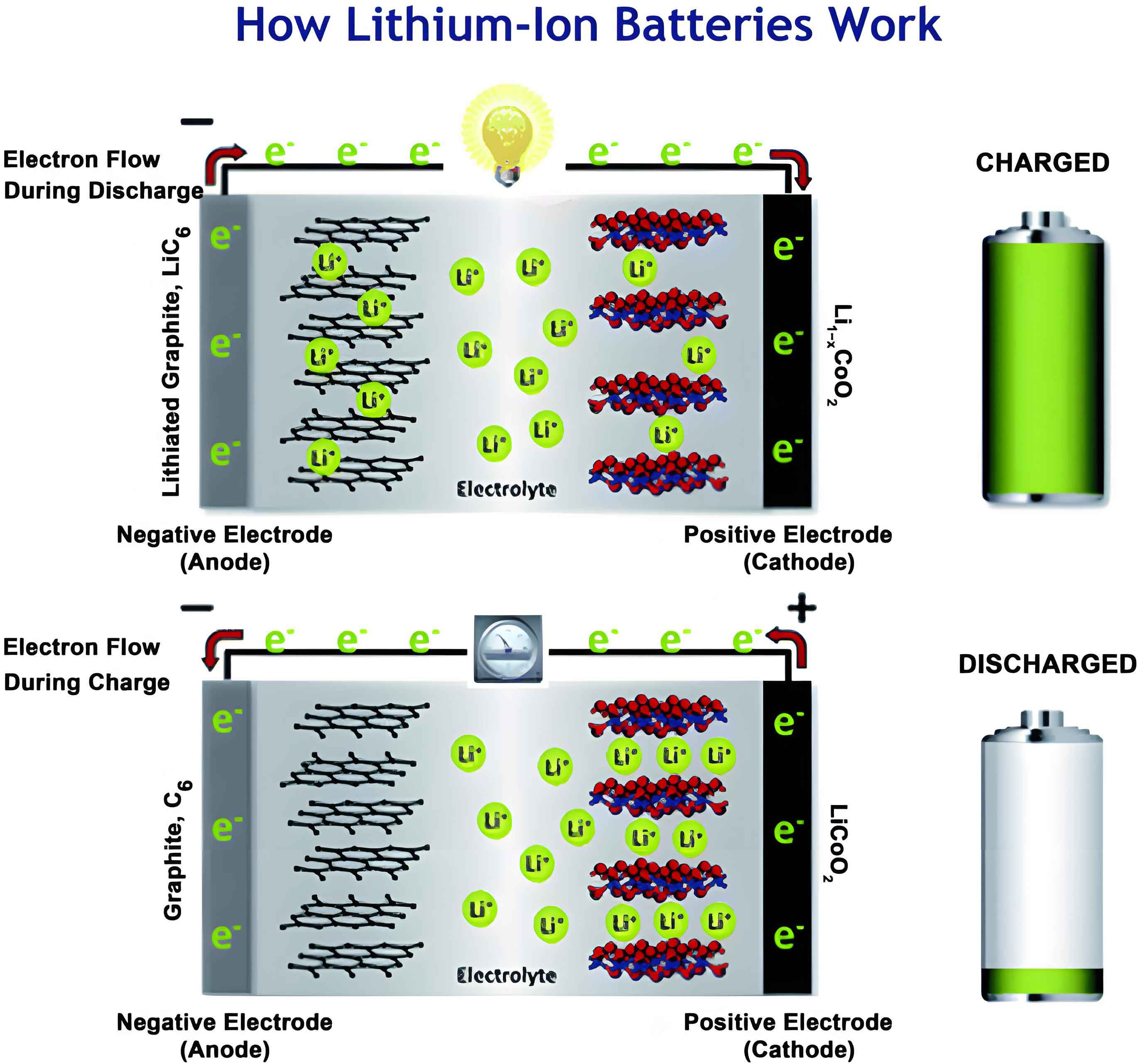
Lithium-ion battery modeling is essential for SOC estimation, with common approaches including electrochemical, black-box, and equivalent circuit models. The equivalent circuit model (ECM) is widely adopted for its simplicity, interpretability, and ability to capture dynamic behaviors. Among ECMs, the second-order RC model is preferred as it accounts for both electrochemical polarization and concentration polarization, providing a balance between accuracy and computational efficiency. This model consists of an ohmic resistor, two RC parallel networks, and an open-circuit voltage (OCV) source, where the OCV is a nonlinear function of SOC. The governing equations for the second-order RC model are derived from Kirchhoff’s laws, leading to state-space representations that facilitate SOC estimation. The state variables typically include polarization voltages and SOC, while the terminal voltage serves as the observation. The dynamics can be expressed as:
$$U_{T,k} = U_{OC} – I_k R_0 – U_{1,k} – U_{2,k}$$
$$U_{1,k+1} = U_{1,k} e^{-\frac{\Delta t}{\tau_1}} + I_{k+1} R_1 \left(1 – e^{-\frac{\Delta t}{\tau_1}}\right)$$
$$U_{2,k+1} = U_{2,k} e^{-\frac{\Delta t}{\tau_2}} + I_{k+1} R_2 \left(1 – e^{-\frac{\Delta t}{\tau_2}}\right)$$
where \(U_{T,k}\) is the terminal voltage at time \(k\), \(U_{OC}\) is the open-circuit voltage, \(I_k\) is the current, \(R_0\) is the ohmic resistance, \(U_{1,k}\) and \(U_{2,k}\) are polarization voltages, \(\tau_1 = R_1 C_1\) and \(\tau_2 = R_2 C_2\) are time constants, and \(\Delta t\) is the sampling interval. The state-space formulation is:
$$\begin{bmatrix} U_{1,k} \\ U_{2,k} \\ SOC_k \end{bmatrix} = \begin{bmatrix} e^{-\frac{\Delta t}{\tau_{1,k-1}}} & 0 & 0 \\ 0 & e^{-\frac{\Delta t}{\tau_{2,k-1}}} & 0 \\ 0 & 0 & 1 \end{bmatrix} \begin{bmatrix} U_{1,k-1} \\ U_{2,k-1} \\ SOC_{k-1} \end{bmatrix} + \begin{bmatrix} I_{k-1} R_{1,k-1} \left(1 – e^{-\frac{\Delta t}{\tau_1}}\right) \\ I_{k-1} R_{2,k-1} \left(1 – e^{-\frac{\Delta t}{\tau_2}}\right) \\ -\frac{\eta \Delta t}{C_N} \end{bmatrix} + \begin{bmatrix} \omega_{U_1,k-1} \\ \omega_{U_2,k-1} \\ \omega_{SOC,k-1} \end{bmatrix}$$
$$U_{T,k} = U_{OC}(SOC_k) + [-1 \ -1 \ 0] \begin{bmatrix} U_{1,k} \\ U_{2,k} \\ SOC_k \end{bmatrix} – R_0 I_k + v_k$$
where \(SOC_k\) is the state of charge, \(\eta\) is coulombic efficiency, \(C_N\) is nominal capacity, \(\omega_k\) is process noise, and \(v_k\) is measurement noise. This model forms the basis for parameter identification and SOC estimation, crucial for managing lithium-ion battery systems.
Parameter identification is vital for accurate modeling of lithium-ion batteries, as parameters like resistances and capacitances vary with SOC, temperature, and aging. Traditional methods like recursive least squares (RLS) may suffer from data saturation, leading to poor tracking of time-varying parameters. To overcome this, the adaptive forgetting factor recursive least squares (AFFRLS) algorithm is employed. It introduces a dynamic forgetting factor that adjusts based on estimation errors, enhancing convergence and stability. The AFFRLS algorithm steps are as follows:
- Initialize parameters: \(\lambda_{min} = 0.98\), \(e_{base} = 0.001\), \(h = 0.9\), \(\theta(0) = \frac{1}{\delta} [1, 1, 1]^T\), \(P_0(0) = \delta I_0\), where \(\delta\) is a large positive number and \(I_0\) is identity matrix.
- Compute estimation error: \(e(k) = y(k) – \varphi^T(k) \theta(k)\).
- Calculate gain matrix: \(K_0(k+1) = \frac{P_0(k) \varphi(k+1)}{\lambda + \varphi(k+1)^T P_0(k) \varphi(k+1)}\).
- Update parameter vector: \(\theta(k+1) = \theta(k) + K_0(k+1) [y(k+1) – \varphi^T(k+1) \theta(k)]\).
- Update covariance matrix: \(P_0(k+1) = \frac{1}{\lambda} [I – K_0(k+1) \varphi^T(k+1)] P_0(k)\).
- Adapt forgetting factor: \(\lambda(k) = \lambda_{min} + (1 – \lambda_{min}) h^{\varepsilon(k)}\), where \(\varepsilon(k) = \text{round} \left( \frac{e^T(k)}{e_{base}} \right)^2\).
- Repeat from step 2 for each time instance.
This approach allows the AFFRLS algorithm to maintain accuracy under varying conditions for lithium-ion batteries, as the forgetting factor decreases when errors are large to speed up convergence and approaches 1 when errors are small to ensure stability. The algorithm is applied to identify parameters such as \(R_0\), \(R_1\), \(R_2\), \(C_1\), and \(C_2\) in real-time, using terminal voltage and current measurements from lithium-ion battery tests.
For SOC estimation, the adaptive unscented Kalman filter (AUKF) is utilized to handle nonlinearities and noise uncertainties in lithium-ion battery systems. Unlike standard UKF, AUKF incorporates covariance matching to online adjust process and measurement noise covariances, improving robustness. The AUKF algorithm involves the following steps for a discrete nonlinear system:
State and observation equations: \(x_k = f(x_{k-1}, u_{k-1}) + w_k\), \(y_k = g(x_k, u_k) + v_k\), where \(x_k\) is state vector (including SOC), \(y_k\) is output, \(w_k\) and \(v_k\) are noises with covariances \(Q_k\) and \(R_k\).
- Initialize: \(\hat{x}_{0|0} = E[x_0]\), \(P_{xx,0|0} = E[(x_0 – \hat{x}_0)(x_0 – \hat{x}_0)^T]\), \(R_0\), \(Q_0\).
- Generate sigma points: for \(i=0\), \(\hat{x}^{(0)}_{k-1|k-1} = \hat{x}_{k-1|k-1}\); for \(i=1,\ldots,n\), \(\hat{x}^{(i)}_{k-1|k-1} = \hat{x}_{k-1|k-1} + \sqrt{(n+\lambda) P_{xx,k-1|k-1}}\); for \(i=n+1,\ldots,2n\), \(\hat{x}^{(i)}_{k-1|k-1} = \hat{x}_{k-1|k-1} – \sqrt{(n+\lambda) P_{xx,k-1|k-1}}\), where \(\lambda = \alpha^2 (n+\kappa) – n\), with \(\alpha\) and \(\kappa\) tuning parameters.
- Time update: propagate sigma points: \(\hat{x}^{(i)}_{k|k-1} = f(\hat{x}^{(i)}_{k-1|k-1}, u_{k-1})\), compute predicted state: \(\hat{x}_{k|k-1} = \sum_{i=0}^{2n} \omega_i^m \hat{x}^{(i)}_{k|k-1}\), and predicted covariance: \(P_{xx,k|k-1} = \sum_{i=0}^{2n} \omega_i^c (\hat{x}^{(i)}_{k|k-1} – \hat{x}_{k|k-1})(\hat{x}^{(i)}_{k|k-1} – \hat{x}_{k|k-1})^T + Q_k\), with weights \(\omega_0^m = \frac{\lambda}{n+\lambda}\), \(\omega_0^c = \frac{\lambda}{n+\lambda} + (1-\alpha^2+\beta)\), and \(\omega_i^m = \omega_i^c = \frac{1}{2(n+\lambda)}\) for \(i=1,\ldots,2n\).
- Measurement update: predict observations: \(\hat{y}^{(i)}_{k|k-1} = g(\hat{x}^{(i)}_{k|k-1}, u_k)\), compute predicted output: \(\hat{y}_{k|k-1} = \sum_{i=0}^{2n} \omega_i^m \hat{y}^{(i)}_{k|k-1}\), output covariance: \(P_{yy,k|k-1} = \sum_{i=0}^{2n} \omega_i^c (\hat{y}^{(i)}_{k|k-1} – \hat{y}_{k|k-1})(\hat{y}^{(i)}_{k|k-1} – \hat{y}_{k|k-1})^T + R_k\), and cross-covariance: \(P_{xy,k|k-1} = \sum_{i=0}^{2n} \omega_i^c (\hat{x}^{(i)}_{k|k-1} – \hat{x}_{k|k-1})(\hat{y}^{(i)}_{k|k-1} – \hat{y}_{k|k-1})^T\).
- Compute Kalman gain: \(K_k = P_{xy,k|k-1} P_{yy,k|k-1}^{-1}\).
- Update state estimate: \(\hat{x}_{k|k} = \hat{x}_{k|k-1} + K_k (y_k – \hat{y}_{k|k-1})\).
- Update state covariance: \(P_{xx,k|k} = P_{xx,k|k-1} – K_k P_{yy,k|k-1} K_k^T\).
- Adapt noise covariances using covariance matching: \(H_k = \frac{1}{N} \sum_{i=k-M+1}^{k} e_k e_k^T\), where \(e_k = y_k – \hat{y}_{k|k-1}\), then update \(R_k = H_k – C_k P_{xx,k|k-1} C_k^T\) and \(Q_k = K_k H_k K_k^T\), with \(C_k = \left. \frac{\partial g(x, u_k)}{\partial x} \right|_{x = \hat{x}_{k|k-1}}\).
This AUKF algorithm, combined with AFFRLS for parameter identification, forms the AFFRLS-AUKF joint method for SOC estimation in lithium-ion batteries. The integration allows real-time adaptation to parameter changes and noise statistics, crucial for accurate SOC tracking under dynamic loads.
Experimental validation is conducted using publicly available lithium-ion battery datasets, covering multiple driving cycles such as DST, FUDS, US06, and BJDST to simulate real-world conditions. The lithium-ion battery used is a common cylindrical type, with tests performed at room temperature. The AFFRLS algorithm is applied for online parameter identification, with results showing time-varying trends in \(R_0\), \(R_1\), \(R_2\), \(C_1\), and \(C_2\) across different cycles. The forgetting factor \(\lambda\) adjusts dynamically, indicating the algorithm’s responsiveness to changes in lithium-ion battery behavior. For instance, under DST cycle, parameters fluctuate with current variations, while under FUDS, more severe polarization effects are observed. The identified parameters are then used in the second-order RC model to predict terminal voltage, with errors analyzed to verify identification accuracy.
The SOC estimation performance of the AFFRLS-AUKF method is evaluated by comparing estimated SOC with reference values obtained from coulomb counting or other benchmarks. Results under each operating condition demonstrate high accuracy. For example, under DST, the SOC estimates closely follow the reference with minimal deviation. The errors are quantified using mean absolute error (MAE) and root mean square error (RMSE), as summarized in the table below.
| Operating Condition | Mean Absolute Error (MAE) | Root Mean Square Error (RMSE) |
|---|---|---|
| DST | 0.0035 | 0.0095 |
| FUDS | 0.0110 | 0.0138 |
| US06 | 0.0011 | 0.0109 |
| BJDST | 0.0077 | 0.0176 |
The table indicates that the AFFRLS-AUKF method achieves low errors across all cycles, with MAE below 0.0110 and RMSE below 0.0176, highlighting its effectiveness for lithium-ion battery SOC estimation. Notably, under US06, the MAE is as low as 0.0011, showcasing superior precision. These results are attributed to the adaptive capabilities of both AFFRLS and AUKF, which handle parameter variations and noise uncertainties inherent in lithium-ion batteries. Additionally, the method’s robustness is confirmed by consistent performance under diverse loads, from urban driving to highway cycles.
Further analysis involves comparing the proposed method with traditional approaches like fixed-parameter RLS or standard UKF. The AFFRLS-AUKF method shows significant improvements in tracking accuracy and convergence speed, especially during transient phases where lithium-ion battery parameters change rapidly. For instance, during high-current pulses, the adaptive forgetting factor ensures quick parameter updates, while AUKF’s noise adaptation mitigates estimation drift. This synergy enhances the overall reliability of SOC estimation for lithium-ion battery management systems.
In conclusion, this paper presents a novel joint algorithm based on AFFRLS and AUKF for SOC estimation of lithium-ion batteries under multiple operating conditions. The second-order RC model provides a balance between complexity and accuracy, while AFFRLS enables real-time parameter identification with adaptive forgetting, and AUKF offers robust state estimation with noise covariance matching. Experimental results validate the method’s high accuracy, with MAE values as low as 0.0035 for DST, 0.0110 for FUDS, 0.0011 for US06, and 0.0077 for BJDST cycles. The algorithm effectively addresses challenges such as time-varying parameters and noise in lithium-ion batteries, ensuring reliable SOC estimation for enhanced battery longevity and system efficiency. Future work could explore integration with thermal models or aging effects to further improve lithium-ion battery management.
The proposed AFFRLS-AUKF method demonstrates strong generalization across different driving profiles, making it suitable for practical applications in electric vehicles and energy storage systems. By leveraging adaptive techniques, it overcomes limitations of conventional methods and sets a foundation for advanced BMS development. Continued research on lithium-ion battery modeling and estimation will contribute to safer and more efficient utilization of lithium-ion battery technologies in the renewable energy landscape.