
In recent years, the global energy crisis and environmental degradation have intensified the demand for clean and sustainable energy sources. Photovoltaic (PV) power generation, as a key technology in the renewable energy sector, has witnessed rapid growth due to its potential to reduce carbon emissions and reliance on fossil fuels. However, PV systems face challenges such as high initial costs, relatively low conversion efficiency of solar cells, and environmental concerns associated with the manufacturing process of silicon wafers. Additionally, the output characteristics of PV modules are inherently nonlinear and highly dependent on solar irradiance and ambient temperature, making it impractical to model them simply as DC voltage sources. This paper focuses on developing a robust simulation model for an off-grid solar system, specifically a two-stage single-phase configuration, using MATLAB/Simulink. By leveraging the Subsystem and S-function builder modules, along with C language programming, we simplify the mathematical modeling of solar cells and create an enhanced PV module simulation. This model accurately replicates the I-V and P-V characteristics under varying irradiance and temperature conditions without requiring intricate internal cell parameters. Furthermore, we integrate a Boost converter for DC-DC conversion and a voltage hysteresis tracking technique for inverter control, resulting in a stable and efficient off-grid solar system simulation. The findings contribute to the optimization and design of practical off-grid solar systems, which are crucial for remote and standalone applications.
The core of any off-grid solar system lies in the accurate representation of PV modules, which convert sunlight directly into electricity through the photovoltaic effect. A typical PV cell consists of a p-n junction formed by doping silicon with elements like boron (p-type) and phosphorus (n-type). When photons strike the junction, they generate electron-hole pairs, leading to a potential difference and current flow. The equivalent circuit of a solar cell, as shown in Figure 1, includes a current source representing photocurrent, a diode for the p-n junction, series resistance (Rs), and shunt resistance (Rsh). The output current I of a single cell can be expressed as:
$$ I = I_{ph} – I_0 \left[ \exp\left(\frac{q(V + I R_s)}{A K T}\right) – 1 \right] – \frac{V + I R_s}{R_{sh}} $$
where I_ph is the photocurrent, I_0 is the reverse saturation current, q is the electron charge (1.602 × 10^{-19} C), K is Boltzmann’s constant (1.38065 × 10^{-23} J/K), A is the diode ideality factor, T is the cell temperature in Kelvin, V is the output voltage, and R_s and R_sh are the series and shunt resistances, respectively. For a PV module comprising n cells in series, the output voltage V1 and current I1 are derived from the generalized equation:
$$ V_1 = \frac{A K T}{q} \ln\left( \frac{I_{ph1} – I_1 – I_{sh}}{I_0} + 1 \right) + \cdots + \frac{A K T}{q} \ln\left( \frac{I_{phn} – I_1 – I_{sh}}{I_0} + 1 \right) – n I_1 R_s $$
with the shunt current I_sh given by:
$$ I_{sh} = \frac{V_1 + n I_1 R_s}{n R_{sh}} $$
Under ideal conditions, assuming uniform photocurrent I_ph across cells and neglecting the shunt current due to high R_sh, the simplified output current equation becomes:
$$ I_1 = I_{sc} – I_0 \left[ \exp\left(\frac{q(V_1 + I_1 R_{s1})}{A_1 K T}\right) – 1 \right] $$
where I_sc is the short-circuit current under standard test conditions (STC: 1000 W/m² irradiance and 25°C), R_s1 is the module series resistance, and A_1 is the module diode factor. Using nameplate data from PV modules, such as open-circuit voltage (V_oc), short-circuit current (I_sc), and maximum power point (MPP) values (V_m and I_m), the model can be parameterized with coefficients C1 and C2:
$$ I_1 = I_{sc} \left[ 1 – C_1 \left( \exp\left(\frac{V_1}{C_2 V_{oc}}\right) – 1 \right) \right] $$
where:
$$ C_1 = \left(1 – \frac{I_m}{I_{sc}}\right) \exp\left(-\frac{V_m}{C_2 V_{oc}}\right) $$
$$ C_2 = \left(\frac{V_m}{V_{oc}} – 1\right) \left[ \ln\left(1 – \frac{I_m}{I_{sc}}\right) \right]^{-1} $$
To account for environmental variations, the IEC 60891-2009 standard provides correction formulas for changes in irradiance and temperature. The current and voltage deviations, ΔI and ΔV, are calculated as:
$$ \Delta I = I_{sc} \left( \frac{G_2}{G_1} – 1 \right) + \alpha (T_2 – T_1) $$
$$ \Delta V = -R_{s1} \Delta I + \beta (T_2 – T_1) $$
where G_1 and T_1 are STC irradiance and temperature, G_2 and T_2 are arbitrary conditions, and α and β are the current and voltage temperature coefficients, respectively. Thus, the final I-V equation for a PV module under non-STC conditions is:
$$ I_1 = I_{sc} \left[ 1 – C_1 \left( \exp\left(\frac{V_1 + \Delta V}{C_2 V_{oc}}\right) – 1 \right) \right] + \Delta I $$
In Simulink, this mathematical model is implemented using a Subsystem block and an S-function builder with C code for efficient computation. The PV module is treated as a controllable current source, and the S-function handles the real-time calculation of output current based on input irradiance and temperature. This approach allows for dynamic simulation of I-V and P-V curves under varying conditions, as demonstrated in Figure 5, where curves remain smooth and stable with reduced simulation step sizes. The model’s versatility extends to simulating PV strings and arrays by scaling parameters appropriately.
| Parameter | Symbol | Value |
|---|---|---|
| Short-circuit current | I_sc | 8.5 A |
| Open-circuit voltage | V_oc | 36 V |
| Maximum power voltage | V_m | 29 V |
| Maximum power current | I_m | 8.0 A |
| Series resistance | R_s | 0.05 Ω |
| Shunt resistance | R_sh | 1000 Ω |
| Temperature coefficient of I_sc | α | 0.05 %/°C |
| Temperature coefficient of V_oc | β | -0.3 %/°C |
For the two-stage off-grid solar system, the first stage involves a DC-DC Boost converter to elevate the PV array voltage to a level suitable for inversion. The Boost converter operates by controlling a MOSFET switch with pulse-width modulation (PWM), adjusting the duty cycle D to maintain the input impedance match for maximum power point tracking (MPPT). The input-output relationship is given by:
$$ \frac{V_i}{I_i} = R_{out} (1 – D)^2 $$
where V_i and I_i are the input voltage and current, and R_out is the output resistance. An improved perturb and observe (P&O) MPPT algorithm is employed, which samples the PV array’s output voltage and current, computes the power, and compares it with previous values to determine the perturbation direction. The cumulative perturbation step is compared with a sawtooth carrier signal to generate PWM pulses, ensuring precise tracking of the MPP even under rapidly changing conditions. The MPPT control model in Simulink, as depicted in Figure 8, utilizes relays, memory blocks, and logical operators to implement this logic. Simulation results under STC and real-world varying conditions (Figure 10) show stable tracking, with power output adapting to irradiance and temperature fluctuations, such as the decline in power during periods of decreasing irradiance.
| Component | Parameter | Value |
|---|---|---|
| Boost Inductor | L | 1.5 mH |
| Output Capacitor | C | 1000 μF |
| Switching Frequency | f_sw | 20 kHz |
| MPPT Perturbation Step | ΔD | 0.01 |
| PV Array Configuration | Series-Parallel | 2 strings × 9 modules |
The second stage of the off-grid solar system is the DC-AC inversion, achieved through a voltage hysteresis tracking PWM inverter. This technique uses a closed-loop control where the load voltage feedback is compared with a sinusoidal reference signal V_ref (311 V peak, 50 Hz). The hysteresis comparator with a band width of 2ΔU generates PWM signals to control the IGBTs in a full-bridge configuration, ensuring the output voltage tracks V_ref within the tolerance band. The output voltage V is filtered through an LC filter (L1 = 1.5 mH, C3 = 30 μF) to attenuate high-frequency harmonics. The resulting AC voltage and current waveforms, shown in Figure 12, exhibit low total harmonic distortion (THD = 1.07%), meeting standards like GB/T 19964-2012. Discrete Fourier analysis (Figure 13) confirms minimal harmonic content, with the fundamental component at 50 Hz dominating the output.
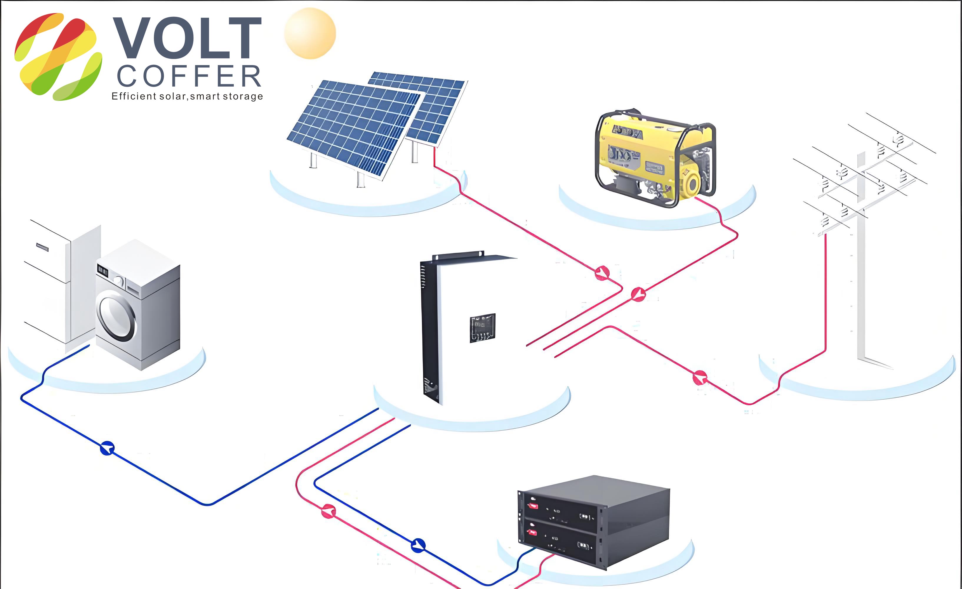
The simulation of the entire two-stage single-phase off-grid solar system integrates the PV array model, Boost converter, MPPT control, and inverter into a cohesive Simulink environment. The system demonstrates robustness under dynamic conditions, such as variations in solar irradiance and temperature, which are critical for real-world off-grid applications. By employing the improved P&O MPPT method and voltage hysteresis tracking, the system maintains high efficiency and stability, reducing the need for complex hardware iterations. This modeling approach provides a valuable tool for designing and optimizing off-grid solar systems, particularly in remote areas where grid connectivity is unavailable. Future work could explore integration with energy storage systems and advanced control strategies to enhance reliability and scalability.
In summary, this paper presents a comprehensive simulation framework for a two-stage single-phase off-grid solar system using Simulink. The PV module model, based on mathematical equations and C code implementation, accurately captures nonlinear characteristics under varying environmental conditions. The Boost converter with MPPT ensures optimal power extraction, while the voltage hysteresis inverter delivers high-quality AC output. The results validate the model’s effectiveness, offering insights for practical deployments of off-grid solar systems in sustainable energy solutions.