
In order to achieve carbon peaking and carbon neutrality goals as soon as possible, new energy sources with strong random fluctuations have been rapidly developed, resulting in increasingly serious peak valley load differences in the power grid. To improve the stability and safety of power grid operation, it is necessary to introduce corresponding peak shaving and valley filling measures. Relying solely on the complementary and interdependent regulation of multiple energy sources often has limitations. The volatility and randomness of new energy sources can pose challenges to the stability and safety of the power grid, and on the other hand, it is detrimental to the energy consumption itself. Therefore, configuring energy storage in the power grid to improve the system’s regulation capacity is an effective and necessary measure. The coordinated scheduling of source, network, load, and storage combined with the energy internet is an effective measure to achieve efficient utilization of new energy and load shaving and valley filling of the power grid.
The traditional peak shaving method adjusts the output power of the power generation units in the grid by observing the load fluctuations of the power grid, requiring them to have a high peak shaving capacity, and frequent start-up and shutdown of units also leads to waste of fuel resources. Compared to this, large-scale battery energy storage systems that are regulated from the load side have more significant advantages in peak shaving and valley filling. On the one hand, there is a large amount of research available for application in the field of optimal scheduling of battery energy storage systems (BESS); On the other hand, the prospect of battery cascade utilization is broad, and the construction cost of battery energy storage systems has been significantly reduced. By comparing the cost and service life of cascaded utilization batteries and new batteries, the relationship between the corresponding energy storage system benefits and factors such as battery purchase price and peak valley electricity price difference was studied. On the basis of such research, the application scope and economy of battery energy storage systems have been greatly developed. Therefore, in a broader application field, research on the participation of related battery energy storage systems in peak shaving has been carried out. Propose a control strategy that utilizes electric vehicle batteries as energy storage platforms to participate in microgrid peak shaving, improving the operational efficiency of the microgrid by providing buffering for renewable energy within the microgrid. Propose a peak shaving and valley filling optimization scheduling method using energy storage power plants, which optimizes the overall net load variance under the system peak shaving demand caused by large-scale distributed photovoltaic grid connection.
However, the energy storage scheduling strategy obtained solely based on the predicted values of load, renewable energy output, etc. still has shortcomings in dealing with source load volatility. Applying robust optimal strategies to deal with source load volatility uncertainty is an effective method. Numerous studies have focused on robust optimal strategies for energy storage scheduling to address the uncertainty of source and load in different scenarios. Propose a multi-objective robust planning method for thermoelectric coupled micro energy systems considering wind power uncertainty, while considering robust optimization and multi-objective optimization issues for energy storage scheduling. However, similar studies are limited to linear forms or require linear approximation of nonlinear parts, resulting in varying degrees of error, and not all nonlinear optimization objectives are suitable for linear approximation. Different evaluation indicators for peak shaving and valley filling were listed and their characteristics and applicable scenarios were compared, including some non-linear evaluation indicators. In the study of energy storage scheduling considering nonlinear optimization objectives, there is less attention to robust optimization. Considering the uncertainty of photovoltaic output and load, a special sequence set method is used to segment linearize the nonlinear model. Although the results are better than particle swarm optimization algorithm, the transformed mixed integer linear programming problem will increase in scale with the increase of the number of segments. At the same time, such methods cannot cope with situations where the range of decision variables is directly influenced by uncertain factors.
Based on this, this article starts with the robust quadratic optimization problem and studies the application of robust optimization problem solutions with nonlinear optimization objectives and constraints involving different stage variables in energy storage scheduling. The traditional column and constraint generation (C&CG) algorithm is mainly used to solve multi-stage robust linear optimization problems. On the basis of existing research results, this article improves the algorithm to solve the aforementioned types of robust multi-objective optimization problems and demonstrates it. Finally, an improved algorithm is used to solve an energy storage optimal scheduling problem with net load variance as the optimization objective and considering the uncertainty of photovoltaic output and load, to verify the effectiveness of the algorithm.
1.Optimization model for energy storage participating in user side peak shaving and valley filling
1.1 Optimization Objectives
This article considers the participation of energy storage in user side peak shaving and valley filling, while selecting photovoltaic power generation as a representative uncertain new energy to be integrated into the same bus. On the one hand, the operation of the power system requires safety and stability, and energy storage scheduling needs to be optimized to make the user side net load curve after energy storage scheduling relatively flat, in order to reduce the frequent start and stop of backup units, and to consider any fluctuations in load and new energy within a certain range; On the other hand, it is necessary to consider the cost of energy storage scheduling, so that the total maintenance cost and electricity price are within an acceptable range.
1.1 1. Peak shaving and valley filling evaluation objectives
Considering the need to make the optimized user side net load curve smoother, it is more suitable to use the user side net load variance as a peak shaving and valley filling evaluation indicator to represent the overall dispersion of the net load within a specified time. This can reduce the overall fluctuation while balancing the peak valley difference of the user side net load.
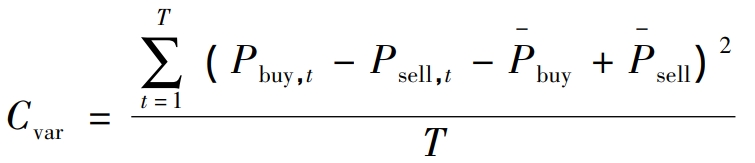
In the formula, Cvar represents the variance of the user side net load; Pbuy, t represents the power purchased by the user side from the power grid at time t; Psell, t represents the power sold by the user to the grid at time t; P-buy is the average value of Pbuy, t within T; P-sell is the average value of Psell, t within T. The user side net load can be expressed as Pbuy, t-Psell, t; T represents the total number of steps in the entire scheduling cycle.
1.1 2 Economic Goals
The total electricity price for purchasing and selling electricity from the external power grid is the main component of the economic goal, as shown in equation (2):
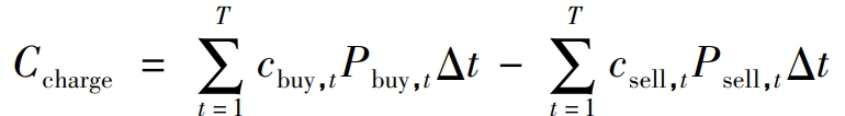
In the formula, Ccharge represents the total electricity price for purchasing and selling electricity from the external power grid; C buy, t and csell, t respectively represent the electricity prices for purchasing and selling electricity. When the model adopts a time of use electricity price, the electricity prices at different times t will change over time based on local specific electricity price policies; Δ T represents the step size.
The maintenance cost considered in this article includes the maintenance cost of energy storage equipment and the maintenance cost of power generation equipment, as shown in equation (3):
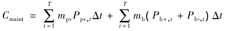
In the formula, C main represents the total maintenance cost; MPV is the maintenance cost coefficient of photovoltaic equipment; Ppv, t represents the output of the photovoltaic equipment at time t; Mb is the maintenance cost coefficient of energy storage equipment; Pb+, t represents the charging power of the energy storage device at time t; Pb -, t represents the discharge power of the energy storage device at time t.
1.2 Constraints
1.2 1 Constraints of battery energy storage system
There are upper and lower limits to the input and output power of the battery energy storage system:
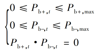
In the formula: Pb+, max represents the upper limit of the charging power of the battery energy storage system; Pb -, max represents the upper limit of the discharge power of the battery energy storage system. The battery energy storage system should minimize internal friction and maintenance costs as much as possible, and constrain Pb+, t · Pb -, t=0 to ensure that at least one charging and discharging power is 0 at the same time.
The state of charge (SOC) of the battery energy storage system must operate within a certain range. On the one hand, it is to extend the service life of the battery; On the other hand, it is to ensure that there is sufficient reserve energy storage to cope with power system failures:
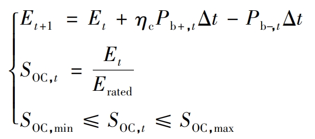
In the formula: Et represents the energy stored by the battery energy storage system at time t; η C represents the energy conversion efficiency; SOC, t represents the state of charge of the battery energy storage system, which needs to operate within a limited range in order for the battery energy storage system to have the expected performance; SOC, min, SOC, max represent the lower and upper bounds of the interval, respectively; Erated represents the total rated capacity of the battery energy storage system.
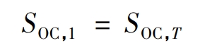
In addition, the energy stored in the battery energy storage system needs to be equal at the beginning and end of an optimization cycle, which makes the impact of the energy stored in the battery energy storage system on any optimization cycle equal, and adjacent optimization cycles can be connected before and after.
1.2 2. Uncertainty Expressed by Box Uncertain Sets
Currently, existing technologies can achieve low error load forecasting, and box uncertainty sets can be used to approximate uncertain quantities with complex or unknown probability distributions. In this article, the uncertainty of load and photovoltaic output is expressed using a box uncertainty set:
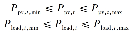
In the formula, Ppv, t, m ax and Ppv, t, min represent the upper and lower bounds of the user side photovoltaic grid connected output power, respectively; Pload, t represents the user side load; Pload, t, m ax and Pload, t, min represent the upper and lower bounds of the user side load, respectively.
For time t, based on the prediction results, the uncertain user side photovoltaic grid connected output power Ppv, t has upper bound Ppv, t, m ax and lower bound Ppv, t, min, and the uncertain user side load Pload, t also fluctuates between upper bound Pload, t, m ax and lower bound Pload, t, min. Because the actual value of the source load cannot be predicted, the energy storage scheduling decision variable must be feasible for any possible fluctuation within the interval, that is, no matter what value the actual value of the source load is taken within the interval, other constraint conditions are met.
1.2.3 Power Equation Constraints
To simplify the model and ignore grid losses, the energy interaction between the user side and the external grid at time t is determined by the photovoltaic power generation, the total load on the user side, and the charging and discharging of the battery energy storage system.

1.3 Construction of Robust Optimization Problems
According to equation (1), construct equation (10) based on the evaluation objective of peak shaving and valley filling to represent the net load variance. The larger the indicator, the more significant the fluctuation in net load.
In the equation, f1 represents the first optimization objective of the robust optimization problem, which is a nonlinear convex function.
According to economic goals, equations (2) and (3) construct equations (11) to represent the total electricity consumption expenditure on the user side.
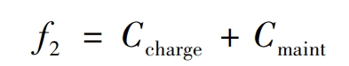
In the equation, f2 represents the second optimization objective of the robust optimization problem, which is a linear function.
Order:
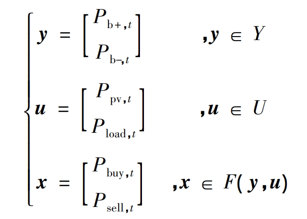
In the formula, y, u, and x are the first stage decision variables, uncertain variables, and second stage decision variables for constructing robust optimization problems through defined variables, respectively; Y. U and F (y, u) are their respective value ranges.
From the constraints of equations (4) to (9), it can be seen that the value range of y, Y set, is a polyhedron independent of u and x. The uncertainty set of u, U set, is a bounded polyhedron independent of y and x. The value range of x, F (y, u), is a polyhedron linearly determined by y and u.
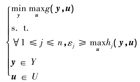
Introduction ε- The constraint method can be used to handle multi-objective optimization problems, and the following robust optimization problems can be constructed:
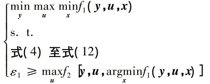
In the equation: ε 1 is for use ε- The specific numerical values required for the constraint method to be given in advance are used to convert the optimization objective f2 into a robust optimization form ε- Constraint, representing the ability of optimization objective f2 when u fluctuates arbitrarily within the U-set
The maximum allowed value.
The purpose of energy storage scheduling is to find a scheduling plan that can meet the constraints of ensuring system security for any possibility of load and photovoltaic fluctuations within an uncertain set, control the economic cost of the system within a certain range, and minimize the net load variance under the most unfavorable scenario.
In equation (13) ε- Constraint representation: after adopting an energy storage scheduling plan y, if u, which is the most unfavorable to f2, is encountered and x is taken according to the principle of minimizing the optimization objective f1, the energy storage scheduling plan y can ensure that f2 can still meet ≤ ε Constraints of 1. The reason is:
1) The specific fluctuation of u is uncontrolled, and once the uncertainty set of the fluctuation is given, it cannot be constrained in any way. Therefore, the constraint of u can limit the value range of y, otherwise it cannot.
2) For a certain energy storage scheduling plan y, although the most unfavorable u for f1 and f2 is generally different, x ∈ F (y, u) does not have two different values for f1 and f2 when y and u are determined. Therefore, the x parameter of f2 in the constraint cannot conflict with f1, and only one value criterion can exist. f2 in the constraint can ultimately be represented as a function h (y, u) of y and u.
2.Improved column and constraint generation algorithm
2.1 Principle and Improvement Scheme of Column and Constraint Generation Algorithm
Define the following linear robust optimization problem:
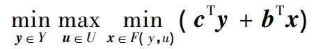
According to the assumption, the first stage decision variable feasible domain Y set is a polyhedron independent of the uncertain variable u and the second stage decision variable x. The uncertain set U set is a polyhedron independent of the first stage decision variable y and the second stage decision variable x. The second stage decision variable feasible domain F (y, u) is a polyhedron determined by y and u. c. Both b are constants, therefore the optimization objective is a linear function. When there are constraints beyond the above forms in the problem, not all elements in the Y and U sets can guarantee the existence of feasible solutions for the second stage decision, that is, when the uncertainty of u can affect the range of y values and cause them to change during the algorithm process, traditional C&CG algorithms will no longer be applicable, and the resulting solutions will have unpredictable errors. The constraint of equation (13) belongs to this type of situation. In addition to the power and SOC related constraints of the battery energy storage system itself, it is required that the economic cost under any possibility in the uncertain concentration is within a given range, which will also affect the feasible region of the scheduling plan. Even if a battery energy storage scheduling plan satisfies the power constraints of the battery energy storage system, as long as there is a possible uncertain scenario that makes the second stage decision unsolvable, the sub problem (SP) of the original algorithm’s search for the most unfavorable scenario will fail due to omitting all uncertain scenarios that make the second stage decision unsolvable. When robust optimization problems involve multiple optimization objectives and more complex multivariable nonlinear constraints, the problem becomes more severe.
The core idea of the original algorithm is to relax the uncertainty set U of the original problem into several scenarios, and enumerate these scenarios to obtain a robust optimal solution that only considers these scenarios, which is the master problem (MP) of the original algorithm. MP is therefore a relaxation problem of the original problem. When MP fails to consider sufficient scenarios, i.e. fails to achieve precise relaxation, as the relaxation problem has more relaxed constraints, the objective function value obtained by MP must not be greater than the optimal objective function value of the original problem. The SP of the original algorithm takes the y obtained from MP as the input of SP, finds the most unfavorable scenario u for the optimization objective in the uncertainty set U, and adds it to several scenarios that MP needs to consider, gradually achieving precise relaxation of the uncertainty set, thereby achieving precise relaxation of MP for the original problem. Because the y used by SP is the solution of MP, which is inferior to the optimal solution of the original problem, the objective function value obtained by SP must not be less than the optimal value of the objective function of the original problem. Repeatedly iterating, SP will continuously supplement the scenarios to be considered by MP until the objective function value obtained by MP is equal to the objective function value obtained by SP. At this point, according to the pinching theorem, the objective function value obtained by MP is equal to the optimal objective function value of the original problem. The several scenarios considered by MP have already achieved precise relaxation of the uncertain set of the original problem, and only considering these scenarios, MP has achieved precise relaxation of the original problem.
However, the original algorithm’s SP can only find the most unfavorable scenario for a single optimization objective in the uncertain set U. Moreover, if the constraints of the SP result in the SP being unable to take values on the complete uncertain set U, then the algorithm will make an error, which is precisely the situation caused by the problem mentioned earlier.
However, if Step 3 is expanded on the basis of the original algorithm and multiple different SP targets that can be simultaneously operated on, this deficiency can be improved. For a class of robust optimization problems shown in equations (12) and (13), this article applies and improves the C&CG algorithm as follows:
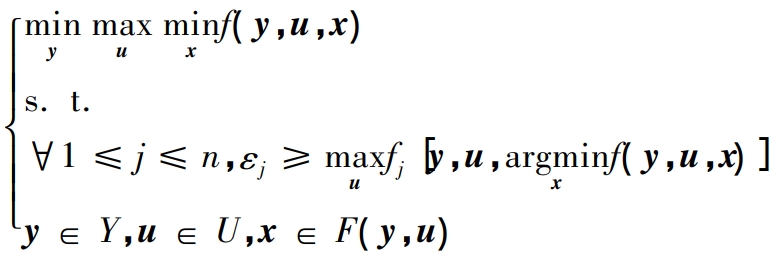
In the formula, the main optimization objective f and the function fj in the constraint conditions are all functions of the first stage decision variable y, the uncertain variable u, and the second stage decision variable x; The Y set is a bounded polyhedron independent of u; The U-set is a bounded polyhedron independent of y; The value range F (y, u) of x is a bounded polyhedron determined by y, u. There are n in total ε- Constraints, where each fj [y, u, argmin xf (y, u, x)] can be represented as a function of y and u, denoted as hj (y, u), and the undefined part of hj (y, u) on the Y and U sets takes a value of+∞.
Step 1: Set Blower=- ∞ and Bubber=+∞ to represent the lower and upper bounds of the optimal value, respectively, and provide the maximum allowable error e. Define the discrete set V, which represents a discrete subset of an uncertain set. Any vertex of U is taken as the initial element of the discrete set V, and its size is initialized to sV=1. Define iteration count k=1.
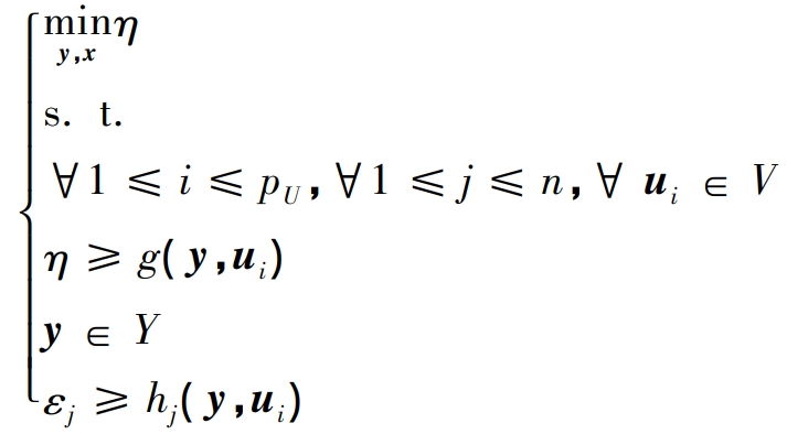
Step 2: Solve MP.
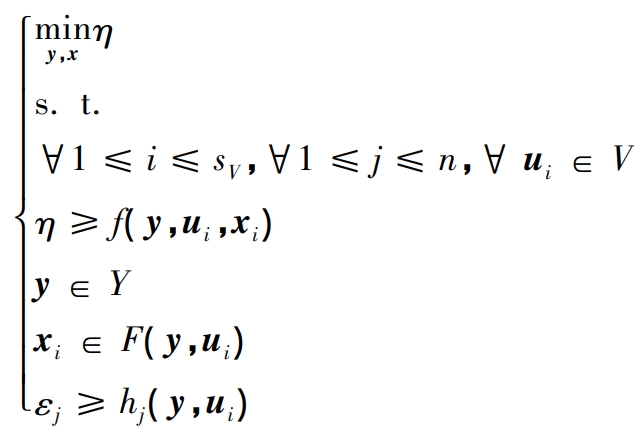
In the equation: η Represents a temporary variable.
Find the optimal solution for MP in the k-th iteration( η* k. Y * k, x * 1,…, x * sV), update Blower= η* K.
The MP here requires the solver to be able to solve nonlinear programming problems:
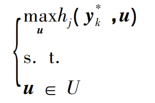
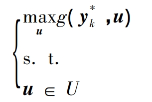
Step 3: Solve n+1 SP separately.
For ∀ 1 ≤ j ≤ n:
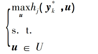
Obtain n sets of optimal solutions (u * k, 1,…, u * k, n) separately.
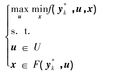
Obtain a set of optimal solutions (u * k, n+1, x * k, n+1).
That is, separately calculate the n+1 scenarios that are most unfavorable for the optimization objective and complex constraints.
If f (y * k, u * k, n+1, x * k, n+1)<Copper and for ∀ 1 ≤ j ≤ n, all satisfy hj (y*
k. U * k, j) < ε J+e, update the Browser to f (y * k, u * k, n+1, x * k, n+1) and record y *=y * k as the current optimal y. If Blower>Bubber e, enter Step 5.
Step 4: Add u * k, n+1 to the discrete set V, and increase its size sV by 1. For ∀ 1 ≤ j ≤ n, if hj (y * k, u * k, j) ≥ ε J+e, then u * k, j are added to the discrete set V, and its size sV increases by 1.
The iteration count k increases by 1. Enter Step 2.
Step 5: Return the current y * as the optimal solution for the robust optimization problem, and end the algorithm.
2.2 The principle and application scope of algorithm improvement
Define the following robust optimization problem:
In the formula: Y set is a bounded polyhedron independent of u; The U-set is a bounded polyhedron independent of y; G (y, u) and hj (y, u) are convex functions.
Proposition 1: If MP has enumerated all vertices of the bounded polyhedron U, then MP is equivalent to the original problem.
In the equation, pU represents the number of vertices of a bounded polyhedron U. If each ui represents a vertex of a bounded polyhedron U, then any element in U can be represented as a convex combination of these vertices ∑ pUi=1
θ I ui( θ I ≥ 0, ∑ pUi=1 θ I=1).
Because g (y, u) is a convex function for u, according to the definition of a convex function, it can be inferred that g (y, ∑ pUi=1 θ I ui) ≤ ∑ pUi=1 θ Ig (y, ui) ≤ ∑ pUi=1 θ I η , That is, under the same conditions, any convex combination of U vertices as a possible scenario in the uncertainty set will not be more detrimental to the optimization objective than all U vertices. Similarly, hj (y, ∑ pUi=1) can be obtained θ I ui) ≤ ∑ pUi=1 θ Ihj (y, ui) ≤ ∑ pUi=1 θ I ε j. If all U vertices satisfy the constraint conditions, then for all possible occurrences of u, the constraint conditions are met. If the MP shown in equation (20) exhausts all vertices of the bounded polyhedron U, then all elements of U satisfy the constraints of MP, which is equivalent to MP considering all elements of U without relaxation, i.e. equivalent to the original problem shown in equation (19).
Proposition 2: In any iteration, there exists a vertex on the bounded polyhedron U that is the solution of SP to the original robust optimization problem shown in equation (19), and unless the algorithm has satisfied the end condition, at least one SP in any iteration will not result in elements that already exist in the discrete set V in the previous iteration.
For ∀ 1 ≤ j ≤ n:
as well as
Equations (21) and (22) represent all SPs of the original robust optimization problem at the k-th iteration. Because g (y, u) is a convex function for u, any convex combination of U vertices, as a possible scenario in the uncertainty set, will not be more detrimental to the optimization objective than all U vertices. Therefore, g (y, ∑ pUi=1 θ I ui) ≤ max 1 ≤ i ≤ pUg (y, ui). Therefore, there always exists a vertex in U that satisfies the optimal condition. Similarly, hj (y, ∑ pUi=1) θ I ui) ≤ max 1 ≤ i ≤ pUhj (y, ui), U always has a vertex that satisfies the optimal condition for that SP.
Let the vertices obtained from n+1 SP be (u * k, 1,…, u * k, n+1). If (u * k, 1,…, u * k, n) are all existing elements in the discrete set V, then they must satisfy the constraints in MP ε J ≥ hj (y * k, u * k, i). In this case, if u * k, n+1 are also existing elements in the discrete set V, then the constraints in MP are also satisfied η* K ≥ g (y * k, u * k, n+1). Therefore, after executing Step 3, it is inevitable that Blower>Bubber e will hold, and the algorithm has met the end condition. Otherwise, at least one element in (u * k, 1,…, u * k, n+1) is not already present in the discrete set V of the previous iteration.
In summary, for the robust optimization problem shown in equation (19), a convergent solution can always be obtained through the above algorithm. In the worst-case scenario, all vertices of the uncertain set U need to be traversed.
Combining equations (10) to (12), such that:
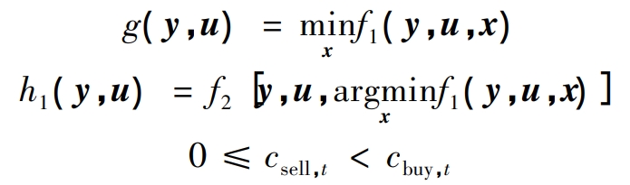
When cbuy, t and csell, t in equation (1) satisfy equation (25), the convexity preserving properties of equation (9) and composite function can ensure that equations (23) and (24) are convex functions. In summary, the robust optimization problem constructed by equation (13) satisfies the requirements of propositions 1 and 2 when equation (25) is satisfied, and can be solved using the algorithm mentioned above.
3.Example analysis
3.1 Specific models and solutions for two optimization objectives
To verify the effectiveness of the proposed strategy, this paper uses MATLAB and Gurobi as simulation tools to establish a user side energy storage scheduling model that includes photovoltaic uncertainty and load uncertainty. In this scenario, in addition to uncontrollable and predictable user loads, there are also uncontrollable and predictable photovoltaic grid connected systems in the microgrid, allowing electricity to be sold to the grid at any time. Taking a residential area as an example,.
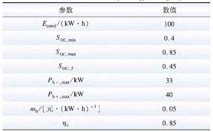
The battery energy storage system in models such as photovoltaic energy storage and idle backup energy storage for base stations that can be used for scheduling adopts cascade utilization of batteries to ensure economic feasibility. Referring to the research, using the parameters shown in Table, it only represents the performance and economic cost of a common type of battery energy storage system constructed by utilizing batteries in a cascade under general operating conditions, and additionally applies SOC constraints to avoid deep charging and discharging to extend its service life, leaving a safety margin.
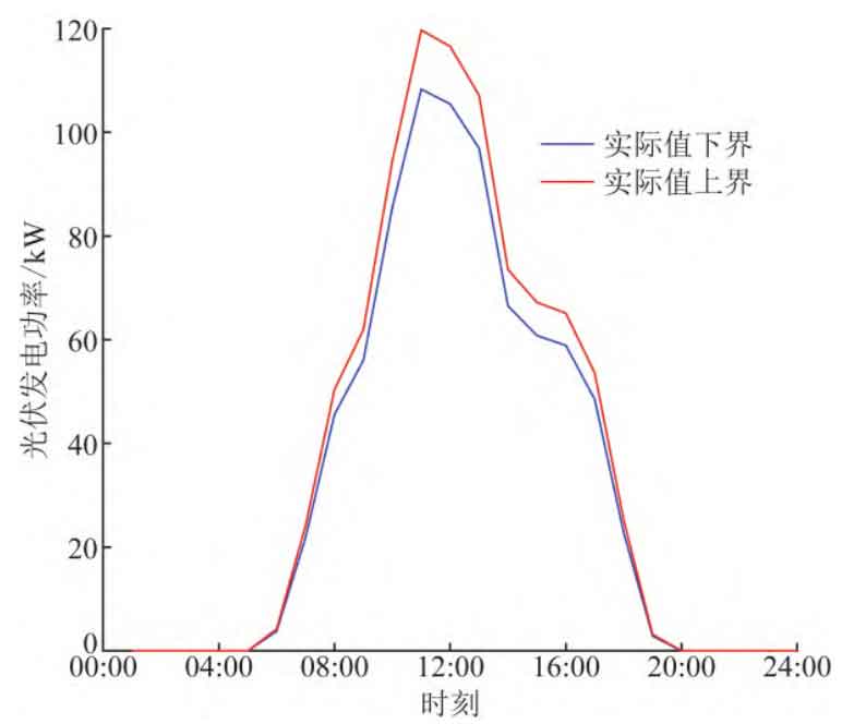
The uncertainty of this model follows the form of equations (7) and (8), as shown in Figures 1 and 2. A feasible energy storage scheduling plan must ensure that all constraints are met regardless of which scenario in the uncertain concentration occurs, i.e., regardless of the value of the source load within this range. The parameters shown in Table meet the requirements of equation (25), so this problem can be solved using 2 The algorithm described in Section 1 is used to solve, and Step3 contains two parallel SPs.
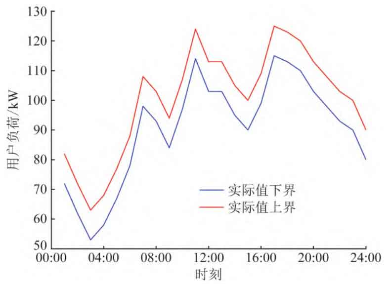
When in equation (13) ε When the value of 1 is 715, that is, after the actual execution of the required energy storage scheduling plan, for any fluctuations in photovoltaic output and user load within the range shown in Figure 1 and Figure 2, all constraints can be met, and the overall electricity consumption expenditure on that day is less than 715 yuan. On this basis, the fluctuation degree of the net load curve on that day should be minimized as much as possible.
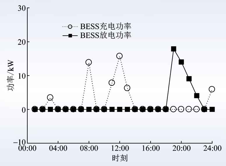
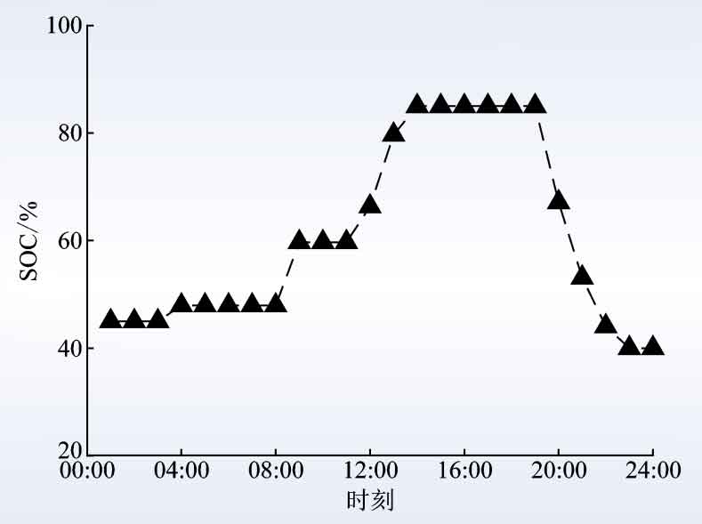
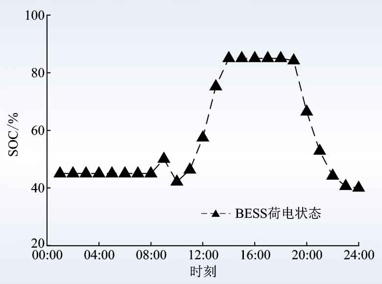
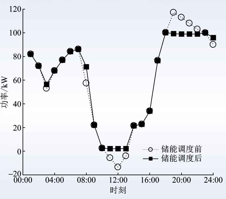
The robust optimal solution of the obtained battery energy storage scheduling plan is shown in Figure 3, and the corresponding SOC changes of the battery energy storage system are shown in Figure 4. For fluctuations in photovoltaic output and user load, even the most unfavorable possibility can meet various constraints of the power system.
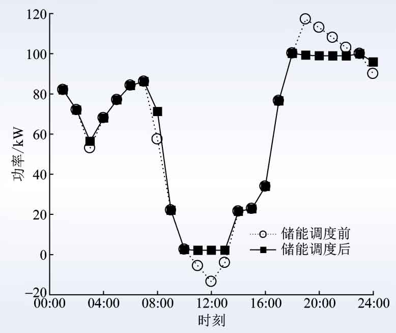
After executing the energy storage scheduling plan, when the most unfavorable possibility of net load variance occurs, the fluctuations in photovoltaic output and user load occur in the most unfavorable form, as shown in Figure 5. At this point, the net load curve without energy storage scheduling is steep and fluctuates greatly, and the energy storage scheduling has the effect of user side peak shaving and valley filling, reducing the degree of fluctuation of the net load curve. In this scenario, the net load variance after energy storage scheduling is 1315 kW2, which is the largest among all possibilities. The total electricity expenditure for that day is 629 yuan, less than the set 715 yuan.
The reason why the total electricity expenditure under the above circumstances did not reach the most unfavorable 715 yuan is because the likelihood of the least favorable net load variance is not the same as the likelihood of the least favorable total electricity expenditure. This issue needs to consider the two most unfavorable possibilities, so we cannot completely sacrifice the total electricity expenditure to optimize the net load variance in the most unfavorable scenario. Moreover, under different energy storage scheduling plans, the two most unfavorable possibilities will become different and need to be determined separately through algorithms, which is also one of the reasons why the improved algorithm requires multiple SPs.
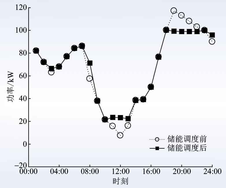
After executing the same energy storage scheduling plan, when the most unfavorable possibility of total electricity expenditure occurs, the energy storage scheduling takes into account the optimization of economic costs while reducing peak load and filling valley on the user side, as shown in Figure 6. Under this possibility, the total electricity expenditure on that day was 715 yuan, reaching the set limit and being the largest of all possibilities; After energy storage scheduling, the net load variance is 784 kW2, which is much smaller than the likelihood of the least favorable net load variance.
This means that if multiple optimization objectives are weighted and summed according to the general optimization problem construction method, the various most unfavorable possible scenarios corresponding to multiple optimization objectives in robust optimization problems will be ignored. Therefore, when considering Pareto optimality in robust optimization problems, it is necessary to avoid the practice of weighted summation of optimization objectives with different dimensions to form new objectives. It is necessary to consider the most unfavorable possible scenario for each optimization objective separately. The source load scenario that is most unfavorable for economic cost objectives can only be used to evaluate the effectiveness of energy storage scheduling in economic cost objectives, and cannot be used to evaluate peak shaving and valley filling objectives, and vice versa. When the maximum acceptable economic cost is determined ε After 1, the optimal peak shaving and valley filling target will be determined accordingly.
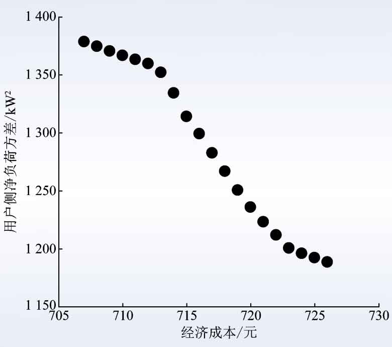
Traverse feasible ε 1. The Pareto front as shown in Figure 7 can be obtained. ε The energy storage scheduling plan with a value of 715 corresponds to an energy storage scheduling plan that is completely biased towards reducing total electricity expenditure, in order to improve the total electricity expenditure under the most unfavorable scenario At the cost of 5%, it reduces the variance of user side net load under the most unfavorable scenario by 9 7%. Compared to energy storage scheduling plans that completely lean towards reducing net load variance, in order to increase the user side net load variance under the most unfavorable scenario by 4 At the cost of 8%, it reduces the total electricity expenditure under the most unfavorable scenario by 1 1%. And for all possible values of uncertain variables in the uncertain set, all energy storage scheduling plans corresponding to the Pareto frontier can ensure that the constraint conditions are met.
The method described in Section 2.1 is not limited to this, and the same method can be applied ε- The constraint method optimizes multiple objectives, which preserves the independent physical meaning of each objective compared to using the weighted sum method to synthesize new objectives, facilitating subsequent analysis and eliminating the discussion of weight selection. The commonly used peak to valley difference of user side net load is now taken as a peak shaving and valley filling evaluation objective that also needs to be considered to further illustrate 2 The method described in Section 1 expands the implementation details of the original algorithm by adding SP.
3.2 Specific models and solutions for multiple optimization objectives
The robust optimization process for multi-objective energy storage scheduling has added an SP for the peak valley difference of user side net load in the Step3 section of the algorithm, which is used to add the most unfavorable scenario in the uncertainty set for the newly added optimization objective to the MP in each iteration. Similarly, inequality constraints involving the first stage decision variables, uncertain variables, and second stage decision variables can be converted even if they do not conform to the prescribed form ε A constant optimization objective constitutes Step 3 of the SP addition algorithm.
When ε 1 value is 720, new target ε When the value of 2 is 92, that is, after the actual execution of the energy storage scheduling plan, it is required to ensure that the photovoltaic output and user load that fluctuate arbitrarily within the range shown in Figure 1 and Figure 2 can meet all constraints, and the overall electricity expenditure on that day is less than 720 yuan, and the peak valley difference of the user side net load is not more than 92 kW. On this basis, the fluctuation degree of the net load curve on that day should be minimized as much as possible.
The robust optimal solution of the battery energy storage scheduling plan obtained under this requirement is shown in Figure 9, and the corresponding SOC changes of the battery energy storage system are shown in Figure 10. From the graph, it can be seen that in order to absorb the peak of photovoltaic power generation at noon and achieve the goal of reducing the peak valley difference, the battery energy storage system discharged from 08:00 to 09:00, reserving capacity for reducing the peak valley.
The user side net load for the most unfavorable scenario of peak to valley net load difference is shown in Figure 11. The newly added SP can search for scenarios with the maximum peak valley difference in user side net load in uncertain sets based on the current energy storage scheduling plan. Under this possibility, the total electricity expenditure on that day is 630 yuan, which is lower than the acceptable upper limit of 720 yuan; The peak to valley difference of the user side net load is 92 kW, which reaches an acceptable upper limit and is the largest among all possible scenarios; The net load variance after energy storage scheduling is 1250 kW2. It can be seen that multiple SPs can balance the composition of multiple objectives ε- Constraints, including inequality constraints involving the first stage decision variables, uncertain variables, and second stage decision variables, can be solved using this method even if they do not conform to the prescribed form.
4.Conclusion
This article focuses on the optimal scheduling problem of user side peak shaving and valley filling energy storage with uncertain source loads. It studies the robust optimization problem and its solution method with the first stage decision value range limited by the second stage decision, and improves the traditional column and constraint generation algorithm. A robust optimal scheduling strategy for battery energy storage with user side peak shaving and valley filling is proposed. The main conclusions are as follows:
1) When the objective function of a single stage robust optimization problem with linear constraints is a convex function, the application of the C&CG algorithm is certain feasible. However, if the uncertainty set in the constraint conditions is not independent of the range of decision variables, the original C&CG algorithm is no longer applicable. For each constraint involving both uncertain sets and decision variables, it can be understood as an application ε- The robust multi-objective optimization problem after the constraint method increases the number of SPs in one iteration of the original C&CG algorithm. As long as these constraints involving both uncertain sets and decision variables are convex function inequalities, the improved algorithm is effective. For two-stage robust optimization problems, it is necessary to prove that when transformed into a single stage robust optimization problem, the innermost function is a convex function, and the constraint conditions involving both uncertain sets and decision variables are convex function inequalities, in order to ensure that the improved algorithm can converge to the robust optimal solution.
2) In the robust optimization problem of energy storage scheduling, due to the significant difference between the most unfavorable scenario for peak shaving and valley filling objectives and the most unfavorable scenario for economic objectives, two scenarios need to be considered separately to obtain a sufficiently conservative robust optimal solution. The algorithm proposed in this paper can balance the impact of uncertain variable fluctuations on the optimization objective and complex constraint conditions. In the case where source load fluctuations affect the feasible range of energy storage output, Effectively solving the robust optimal scheduling problem of battery energy storage for user side peak shaving and valley filling.