
In modern power systems, the integration of renewable energy sources via power electronic converters, particularly on-grid inverters, has become ubiquitous. However, the operational stability and power quality of these on-grid inverters are significantly challenged by the presence of background harmonics in the grid voltage. These harmonics, often introduced by nonlinear loads such as electric trains or industrial machinery, can lead to waveform distortion in the grid-connected current, potentially causing resonance, reducing system efficiency, and compromising grid safety. As an on-grid inverter researcher, I have extensively studied this issue and developed a comprehensive strategy to mitigate such effects. This article presents a detailed analysis of the impact of background harmonics on LCL-type on-grid inverters, proposes a full feed-forward control method for grid voltage, and validates the approach through simulation. The focus is on enhancing the robustness of on-grid inverters in weak grid conditions, ensuring compliance with grid codes such as total harmonic distortion (THD) limits below 5%.
The core of my work involves modeling and controlling a three-phase LCL-type on-grid inverter system. The LCL filter is widely used in on-grid inverters due to its superior harmonic attenuation capabilities compared to simple L filters. However, its resonance characteristics can interact with grid impedance, especially under background harmonic voltages, leading to instability. To address this, I first derive the impedance model of the on-grid inverter system in the stationary αβ reference frame. This model captures the dynamics of the inverter, including the LCL filter, current controller, pulse-width modulation (PWM) delay, and grid interface. By analyzing this model, I elucidate how grid voltage fluctuations, particularly harmonics, propagate to the grid current. The derived expressions reveal that the grid current distortion stems from two main sources: direct disturbance from grid voltage and indirect effects from current reference signals. Understanding these mechanisms is crucial for designing effective suppression strategies.
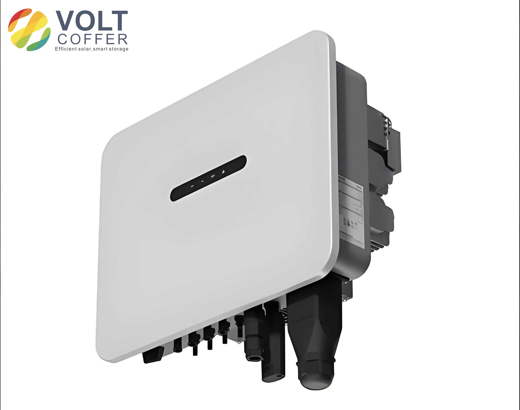
The mathematical modeling begins with the topology of a three-phase LCL-type on-grid inverter. The system comprises a DC voltage source, a three-phase inverter bridge, an LCL filter with inductors L1 and L2 and capacitor C, and a grid connection with line impedance Rg. The control system typically includes a current regulator, a phase-locked loop (PLL) for synchronization, and modulation schemes. For analysis, I consider the α-axis in the stationary frame, where signals are sinusoidal, allowing the use of a quasi-proportional resonant (QPR) controller instead of a PI controller for better AC signal tracking. The transfer function of the QPR controller is given by:
$$G_i(s) = K_p + \frac{2K_r\omega_i s}{s^2 + 2\omega_i s + \omega_1^2},$$
where \(K_p\) is the proportional gain, \(K_r\) is the resonant gain, \(\omega_i\) is the bandwidth, and \(\omega_1 = 2\pi f_1\) with \(f_1 = 50 \, \text{Hz}\) as the grid fundamental frequency. The PWM and inverter bridge are modeled with a gain and delay. The PWM gain is \(G_{\text{PWM}}(s) = U_{in} / (2U_{tri})\), where \(U_{in}\) is the DC-link voltage and \(U_{tri}\) is the carrier amplitude. The delay from digital control, including computation and modulation, is approximated as \(e^{-1.5sT_s}\), where \(T_s\) is the sampling period. Thus, the inverter transfer function becomes:
$$G_{\text{inv}}(s) = \frac{U_{in}}{2U_{tri}} e^{-1.5sT_s}.$$
The PLL dynamics are neglected in high-frequency analysis due to its lower bandwidth relative to the current loop. The control block diagram of the on-grid inverter system in the α-axis is simplified to focus on the current control loop with feedback from capacitor current and grid current. Key parameters are summarized in Table 1, which provides typical values used in simulations.
| Parameter | Symbol | Value |
|---|---|---|
| DC-link voltage | \(U_{dc}\) | 800 V |
| Grid voltage (line-to-line) | \(U_g\) | 380 V |
| Switching frequency | \(f_{sw}\) | 10 kHz |
| Inverter-side inductance | \(L_1\) | 3 mH |
| Grid-side inductance | \(L_2\) | 0.8 mH |
| Filter capacitance | \(C_f\) | 7 µF |
| Line resistance | \(R_g\) | 0.125 Ω |
| Proportional gain | \(K_p\) | 50 |
| Resonant gain | \(K_r\) | 5000 |
| Reference current amplitude | \(I_{dref}\) | 40 A |
From the control block diagram, the output impedance \(Z_o(s)\) of the on-grid inverter is derived as a key metric for stability analysis. The grid current \(i_g(s)\) can be expressed as a function of the reference current \(i_{ref}(s)\) and the grid voltage \(u_{pcc}(s)\) at the point of common coupling (PCC). After simplification, the relationship is:
$$i_g(s) = \frac{T(s)}{1 + T(s)} \frac{1}{K_{i2}} i_{ref}(s) – \frac{G_2(s)}{1 + T(s)} u_{pcc}(s),$$
where \(T(s) = G_1(s)G_2(s)K_{i2}\) is the loop gain, \(G_1(s)\) and \(G_2(s)\) are transfer functions involving the LCL filter and controller, and \(K_{i2}\) is the grid current feedback coefficient. The output impedance is defined as:
$$Z_o(s) = -\frac{u_{pcc}(s)}{i_g(s)} \bigg|_{i_{ref}=0} = \frac{1 + T(s)}{G_2(s)}.$$
This impedance model highlights how the on-grid inverter interacts with the grid. A high output impedance indicates reduced sensitivity to grid voltage disturbances, which is desirable for harmonic suppression. However, the LCL filter introduces resonance peaks that can amplify harmonics at specific frequencies, especially when the grid impedance is weak. To quantify the impact, I analyze the two components of grid current: the disturbance due to grid voltage \(i_{g,v}(s)\) and that due to the reference current \(i_{g,i}(s)\). For \(i_{g,v}(s)\), we have:
$$i_{g,v}(s) = \frac{G_2(s)}{1 + T(s)} u_{pcc}(s) = \frac{1}{Z_o(s)} u_{pcc}(s).$$
This shows that grid voltage harmonics directly inject disturbance currents proportional to the inverse of output impedance. Thus, increasing \(Z_o(s)\) at harmonic frequencies can mitigate this effect. For \(i_{g,i}(s)\), if the loop gain \(T(s)\) is large, the current closely follows the reference, but any harmonics in \(i_{ref}(s)\) will cause distortion. In practice, the reference is often generated from power commands and may contain harmonics due to nonlinearities or grid synchronization errors.
To suppress resonance and harmonic distortion in on-grid inverters, I propose a full feed-forward control strategy for grid voltage. Traditional methods, such as adding resonant controllers or passive damping, have limitations like sensitivity to frequency variations or increased losses. The feed-forward approach directly compensates for grid voltage disturbances without altering the loop gain, thereby preserving stability margins. The derivation starts from the control block diagram, where a feed-forward path is added from the grid voltage measurement to the modulator input. After manipulation, the feed-forward function \(G_f(s)\) is obtained as:
$$G_f(s) = \frac{G_i(s)}{G_1(s)} = \frac{s^2 L_1 C + s C K_{i1} G_{\text{inv}}(s) + 1}{G_{\text{inv}}(s)}.$$
Assuming \(G_{\text{inv}}(s)\) is approximately constant for simplicity, \(G_f(s)\) can be decomposed into three terms: a proportional term \(F_0(s) = 1/G_{\text{inv}}(s)\), a first-derivative term \(F_1(s) = s C K_{i1}\), and a second-derivative term \(F_2(s) = (L_1 C s^2)/G_{\text{inv}}(s)\). In the frequency domain, with \(s = j\omega\), these become:
$$F_1(j\omega) = j\omega C K_{i1}, \quad F_2(j\omega) = -\frac{L_1 C}{G_{\text{inv}}(j\omega)} \omega^2.$$
The full feed-forward thus provides compensation across a broad frequency range, effectively reducing the impact of grid voltage harmonics on the on-grid inverter output current. This strategy is particularly beneficial for weak grids where background harmonics are prevalent. Implementing this in a digital controller requires careful design to avoid introducing additional delays or noise.
To validate the proposed strategy, I conducted simulations in MATLAB/Simulink using the parameters from Table 1. The on-grid inverter system was tested under two scenarios: without background harmonics and with injected harmonics at the PCC. The grid voltage was distorted with typical low-order harmonics (e.g., 5th, 7th, 11th) to simulate realistic conditions. The performance was evaluated based on grid current waveform and THD. Without feed-forward, the on-grid inverter exhibited significant current distortion when background harmonics were present. The THD of the grid current reached 7.03%, exceeding the 5% limit, as shown in Table 2. After enabling the full feed-forward control, the THD dropped to 1.46%, well within the standard, and the current waveform became sinusoidal despite the distorted grid voltage.
| Condition | Grid Current THD | Compliance with 5% Limit |
|---|---|---|
| Without background harmonics | 0.85% | Yes |
| With background harmonics, no feed-forward | 7.03% | No |
| With background harmonics, with full feed-forward | 1.46% | Yes |
The simulation results demonstrate the efficacy of the feed-forward strategy. The mathematical analysis is further supported by frequency-domain plots of the output impedance \(Z_o(s)\). With feed-forward, \(Z_o(s)\) shows increased magnitude at harmonic frequencies, reducing the disturbance current \(i_{g,v}(s)\). This aligns with the principle that enhancing output impedance at critical frequencies suppresses harmonic propagation. The on-grid inverter thus maintains stability and power quality even in weak grid environments. Additional simulations varying grid impedance and harmonic spectra confirm the robustness of the approach for diverse on-grid inverter applications.
In conclusion, background harmonics in grid voltage pose a significant challenge for on-grid inverters, particularly those with LCL filters. Through impedance modeling, I have analyzed the mechanisms by which these harmonics distort grid current. The proposed full feed-forward control strategy effectively mitigates this distortion by compensating for grid voltage disturbances directly. Simulation results show a substantial reduction in THD, from 7.03% to 1.46%, ensuring compliance with grid standards. This strategy enhances the reliability and performance of on-grid inverters in modern power systems. Future work could explore adaptive feed-forward techniques for time-varying harmonic conditions or integration with other advanced control methods for on-grid inverters.
The development of such strategies is crucial as the penetration of renewable energy increases. On-grid inverters must not only convert power efficiently but also actively support grid stability. The full feed-forward method contributes to this goal by improving harmonic immunity without compromising dynamic response. Engineers designing on-grid inverter systems can implement this approach to achieve robust operation in harmonic-rich environments. Continued research in this area will further advance the capabilities of on-grid inverters, facilitating a smoother transition to sustainable energy grids.
To summarize the key equations and parameters, I provide a consolidated list of mathematical expressions used in the analysis. These formulas are essential for designing and tuning on-grid inverter controllers:
- QPR Controller: $$G_i(s) = K_p + \frac{2K_r\omega_i s}{s^2 + 2\omega_i s + \omega_1^2}$$
- Inverter Transfer Function: $$G_{\text{inv}}(s) = \frac{U_{in}}{2U_{tri}} e^{-1.5sT_s}$$
- Output Impedance: $$Z_o(s) = \frac{1 + T(s)}{G_2(s)}$$
- Grid Current Disturbance: $$i_{g,v}(s) = \frac{1}{Z_o(s)} u_{pcc}(s)$$
- Feed-Forward Function: $$G_f(s) = \frac{s^2 L_1 C + s C K_{i1} G_{\text{inv}}(s) + 1}{G_{\text{inv}}(s)}$$
These equations form the foundation for understanding and implementing harmonic suppression in on-grid inverters. By applying them, one can optimize the performance of LCL-type on-grid inverter systems under various grid conditions. The integration of feed-forward control with existing current regulation schemes offers a practical solution for enhancing power quality in real-world applications.