
1. Introduction
With the escalating global environmental challenges and the urgent pursuit of the “dual-carbon” strategic objectives, renewable and clean energy sources are accelerating their transition towards large-scale deployment. In particular, wind power, a critical component of the low-carbon energy architecture, has demonstrated remarkable growth potential. However, the inherent stochasticity and volatility of wind energy pose significant challenges to stable grid integration. This thesis constructs an integrated co-optimization framework that unifies wind power forecasting with energy storage system control. The approach begins with the development of both point and interval forecasting models. Subsequently, leveraging the quantified forecast uncertainty, a rationally sized energy storage system is deployed to provide power compensation, thereby mitigating the randomness associated with wind power. In the grid-connection control phase, model predictive control technology is utilized to suppress wind power fluctuations, ensuring the output power adheres to grid connection specifications.
As the penetration level of wind power continues to climb, the need for reliable forecasting and effective energy storage system control has become paramount. The random nature of wind speed translates directly into fluctuating power outputs, which can destabilize grid frequency and voltage. Energy storage systems present a viable solution to buffer these fluctuations, enabling grid-friendly integration. The synergistic operation of wind farms with energy storage systems is hence recognized as an essential avenue for future energy transformation, providing both technical flexibility and economic viability.
2. Wind Power Point Prediction Based on VMD and GWO-Optimized LSTM
2.1 Background and Rationale
Wind power time series exhibit inherent non-stationarity and complexity. Direct prediction on the raw series often results in substantial errors. To address this, a data preprocessing step employing Variational Mode Decomposition (VMD) is utilized. VMD decomposes the original signal into multiple Intrinsic Mode Functions (IMFs) with varying frequencies, effectively reducing the non-stationarity. Complementing this, the Grey Wolf Optimizer (GWO) is adopted to autonomously optimize the hyperparameters of a Long Short-Term Memory (LSTM) network, which mitigates the inefficiencies and imprecision of manual tuning.
2.2 Methodology
Variational Mode Decomposition (VMD): VMD is a robust, non-recursive signal decomposition technique. The objective is to minimize the total bandwidth of the estimated modes while ensuring the sum of these modes perfectly reconstructs the original signal. The constrained variational problem is formulated as:
$$ \min_{\{u_k\},\{\omega_k\}} \left\{ \sum_{k=1}^{K} \left\| \partial_t \left[ \left( \delta(t) + \frac{j}{\pi t} \right) * u_k(t) \right] e^{-j\omega_k t} \right\|_2^2 \right\} \quad \text{s.t.} \quad \sum_{k=1}^{K} u_k = f $$
Here, \(u_k\) represents the \(k\)-th mode, \(\omega_k\) is its center frequency, and \(f\) is the original signal. The solution is obtained by introducing a quadratic penalty term and Lagrangian multiplier \(\lambda\), leading to the augmented Lagrangian:
$$ \mathcal{L}({u_k},{\omega_k},\lambda) = \alpha \sum_{k=1}^{K} \left\| \partial_t \left[ \left( \delta(t) + \frac{j}{\pi t} \right) u_k(t) \right] e^{-j\omega_k t} \right\|_2^2 + \left\| f(t) – \sum_{k=1}^{K} u_k(t) \right\|_2^2 + \langle \lambda(t), f(t) – \sum_{k=1}^{K} u_k(t) \rangle $$
The Alternating Direction Method of Multipliers (ADMM) is used to iteratively update the modes, their center frequencies, and the Lagrange multiplier to find the optimal solution.
Sample Entropy: To reduce computational overhead and prevent error accumulation, Sample Entropy (\(SE\)) is computed for each decomposed IMF. This metric quantifies the complexity and regularity of a time series. Sequences with similar sample entropy values are reconstructed into a new subsequence, simplifying the modeling process. For a time series of \(N\) points, the sample entropy \(SE\) for a given embedding dimension \(m\) and tolerance \(r\) is calculated as:
$$ SampEn(m, r) = -\ln \frac{A^m(r)}{B^m(r)} $$
Here, \(B^m(r)\) is the probability that two sequences match for \(m\) points within tolerance \(r\), and \(A^m(r)\) is the probability that two sequences match for \(m+1\) points.
Grey Wolf Optimizer (GWO): GWO is a metaheuristic algorithm inspired by the hunting mechanism of grey wolves. The optimization process mimics the leadership hierarchy and hunting behavior of wolf packs. The position update of each wolf is guided by the positions of the top three best solutions (\(\alpha\), \(\beta\), and \(\delta\) wolves). The position of a wolf (\(\vec{X}\)) at iteration \(t\) is updated as follows:
$$ \vec{X}(t+1) = \frac{\vec{X}_1 + \vec{X}_2 + \vec{X}_3}{3} $$
where \(\vec{X}_1\), \(\vec{X}_2\), and \(\vec{X}_3\) are the updated positions based on the \(\alpha\), \(\beta\), and \(\delta\) wolves, respectively. This mechanism ensures effective exploration and convergence to the global optimum.
Long Short-Term Memory (LSTM): LSTM networks are specifically designed to overcome the vanishing/exploding gradient problem common in traditional RNNs. The core of the LSTM cell consists of a forget gate (\(f_t\)), an input gate (\(i_t\)), and an output gate (\(o_t\)). These gates regulate the flow of information through the cell state (\(C_t\)). The key operations are:
$$ f_t = \sigma(W_f [X_t, h_{t-1}] + b_f) $$
$$ i_t = \sigma(W_i [X_t, h_{t-1}] + b_i) $$
$$ C_t = f_t \odot C_{t-1} + i_t \odot \tanh(W_C [X_t, h_{t-1}] + b_C) $$
$$ o_t = \sigma(W_o [X_t, h_{t-1}] + b_o) $$
$$ h_t = o_t \odot \tanh(C_t) $$
2.3 Hybrid VMD-GWO-LSTM Model Development
The proposed hybrid model consists of a sequence of intricate stages. Initially, the raw wind power signal undergoes VMD, resulting in its decomposition into several IMFs. After computing the sample entropy for each, the IMFs are grouped into a smaller set of new sub-series based on entropy similarity. Subsequently, a dedicated LSTM model is constructed for each reconstructed sub-series. The GWO algorithm is then applied to optimize the hyperparameters (specifically, learning rate and hidden layer neuron count) of each LSTM model, training them to attain minimal error. Following the training, the optimal LSTM model is utilized to forecast each sub-series. Ultimately, the predicted values from all sub-series are aggregated additively to derive the final point forecast.
2.4 Case Study and Evaluation
Real-world data from a wind farm in Texas, USA, with a 10-minute sampling interval, was used to validate the model. The dataset was divided into training (80%) and testing (20%) sets. The performance of the VMD-GWO-LSTM model was benchmarked against standard LSTM, GWO-LSTM, and VMD-LSTM models. The evaluation metrics used are the Root Mean Square Error (RMSE), Mean Absolute Error (MAE), and Coefficient of Determination (\(R^2\)).
| Prediction Model | RMSE (MW) | MAE (MW) | \(R^2\) |
|---|---|---|---|
| LSTM | 4.810 | 3.264 | 0.967 |
| GWO-LSTM | 4.514 | 2.966 | 0.971 |
| VMD-LSTM | 2.950 | 2.041 | 0.988 |
| VMD-GWO-LSTM | 2.494 | 1.697 | 0.991 |
The experimental results substantiate the efficacy of the proposed VMD-GWO-LSTM hybrid model. The integration of VMD effectively manages the data complexity, while the GWO optimizes the network hyperparameters, resulting in a combined effect that significantly outperforms the benchmark models. This advanced prediction accuracy forms a robust foundation for the subsequent stages of this research.
3. Interval Prediction Based on Fuzzy C-Means Clustering and Non-parametric Kernel Density Estimation
3.1 Rationale for Interval Forecasting
To fully characterize the uncertainty inherent in wind power forecasting, point prediction alone is insufficient. Interval prediction offers a range of possible outcomes, quantifying the uncertainty associated with the forecast. Building upon the point forecast errors obtained in the previous section, this chapter introduces a method to generate reliable prediction intervals by combining Fuzzy C-Means clustering with non-parametric kernel density estimation.
3.2 Methodology
Fuzzy C-Means Clustering: FCM is a soft clustering algorithm where each data point belongs to every cluster with a certain degree of membership. This is particularly apt for wind power data, which can exhibit characteristics of multiple power regimes. The goal is to partition the dataset \(X = \{x_1, x_2, …, x_N\}\) into \(c\) clusters by minimizing the objective function:
$$ J(X, U, V) = \sum_{i=1}^{N} \sum_{k=1}^{c} u_{ki}^{m_0} d_{ki}^2 $$
Here, \(u_{ki}\) is the membership of data point \(x_i\) in cluster \(k\), \(m_0\) is the fuzziness exponent, and \(d_{ki}\) is the distance between \(x_i\) and the cluster center \(v_k\). The membership and cluster centers are updated iteratively.
Non-parametric Kernel Density Estimation: To model the probability density of forecast errors without assuming a specific parametric distribution, KDE is employed. This data-driven approach is flexible and can capture multi-modal error distributions. The estimated probability density function is given by:
$$ \hat{g}(s) = \frac{1}{N h} \sum_{i=1}^{N} K\left( \frac{s – S_i}{h} \right) $$
where \(S_i\) are the error samples, \(K(\cdot)\) is the kernel function, and \(h\) is the smoothing bandwidth. In this study, the Gaussian kernel is selected, and the bandwidth is dynamically determined via an adaptive algorithm to ensure an optimal balance between bias and variance.
3.3 Model Construction
To construct the interval forecasting model, the point prediction errors are computed. First, the predicted power values are sorted and grouped based on the clustering results from FCM. The fuzzy C-means method identifies the intrinsic patterns within the power data. Then, KDE is applied independently to the forecast errors within each cluster or group. The cumulative distribution function derived from the KDE is then utilized to compute the prediction intervals. For a specified confidence level \((1-\alpha) \times 100\%\), the lower and upper bounds for each error group are determined by the \(\alpha/2\) and \(1-\alpha/2\) quantiles of the cumulative distribution function, respectively.
3.4 Evaluation and Case Study
The performance of the interval prediction model is evaluated using key metrics: Prediction Interval Coverage Probability, Average Interval Width, and the comprehensive score \(F\), which balances both. The \(F\) score is calculated as:
$$ F = \frac{2 \times PICP \times AIW}{PICP + AIW} $$
To validate the proposed FCM-KDE method, it was compared against a traditional KDE approach without the FCM pre-processing step at various confidence levels. The summarized results are presented in the table below.
| Method | Confidence Level (%) | AIW (MW) | PICP | F-score |
|---|---|---|---|---|
| FCM-KDE | 95 | 12.4649 | 0.9513 | 0.1480 |
| 90 | 9.6952 | 0.9026 | 0.1851 | |
| 85 | 7.9906 | 0.8492 | 0.2181 | |
| 80 | 6.9124 | 0.8028 | 0.2449 | |
| KDE | 95 | 12.7109 | 0.9536 | 0.1417 |
| 90 | 9.9301 | 0.9002 | 0.1765 | |
| 85 | 8.0688 | 0.8445 | 0.2112 | |
| 80 | 6.7870 | 0.8071 | 0.2443 |
The findings demonstrate that the FCM-KDE method achieves superior comprehensive performance (indicated by a higher \(F\) value) compared to the conventional KDE technique. These results confirm that the integration of FCM clustering enhances the accuracy and reliability of wind power interval forecasts, providing a more robust reference for grid operations and energy storage system management.
4. Energy Storage System Configuration and SOC Optimization Control
4.1 Strategy for Energy Storage System Sizing Based on Prediction Error Intervals
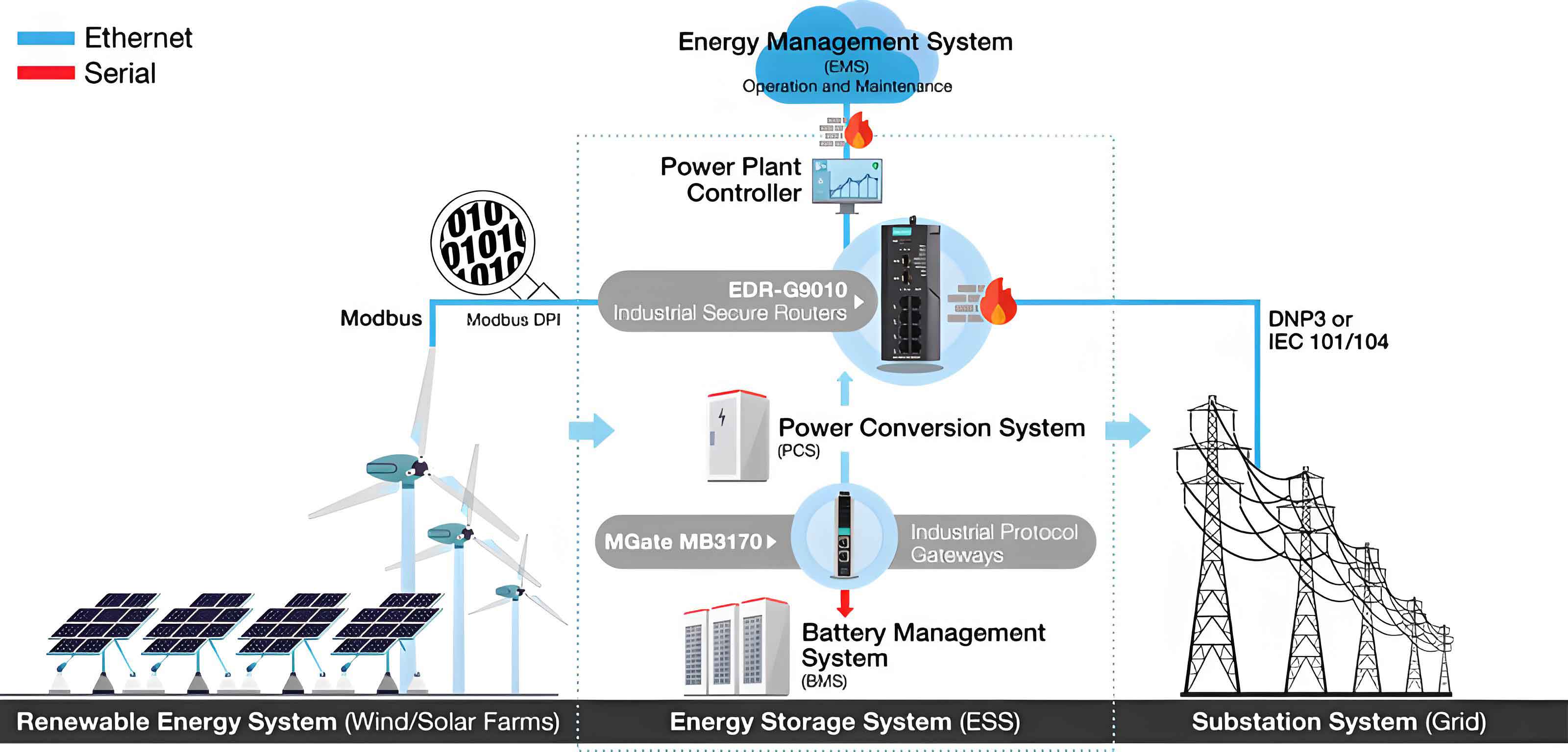
To mitigate the stochasticity of wind power and make wind farm output more predictable, an energy storage system is crucial. This section presents a configuration strategy for the energy storage system based on the prediction error intervals established in Section 3. This strategy aims to control the charging/discharging actions of the energy storage system precisely based on these intervals. When the prediction error is within the bounds of the interval, the energy storage system acts to compensate for the error. Conversely, if the error exceeds the interval, the energy storage system idles, which prevents over-charging or over-discharging and helps to determine an optimal capacity without significant energy waste.
4.2 Capacity and Power Calculation
In a specific approach, the compensation method operates entirely *within* the prediction error interval. The necessary power of the energy storage system is determined by the maximum absolute value of the interval boundaries, while its capacity is calculated based on the energy variations across multiple intervals. The sizing calculations are as follows:
- Rated Power: \( P_r = \text{Max}(|E_u|, |E_l|) \)
where \(E_u\) and \(E_l\) are the upper and lower bounds of the prediction error interval, respectively. - Rated Capacity: The energy storage system’s state of charge (SOC) is bounded between its operational limits \(S_u\) and \(S_l\). The rated capacity \(E_r\) is defined as:
$$ E_r = \frac{\text{max}(E(t)) – \text{min}(E(t))}{S_u – S_l} $$
where \(E(t)\) is the cumulative energy state, reflecting the aggregated power exchange over the operative horizon.
The comparison of energy storage system configurations under different interval forecasting models (as described in Section 3) is presented in Table 4.1. The data clearly show that the choice of forecasting method directly influences the required power and energy capacity.
| Point Prediction Model | Interval Prediction Model | Rated Power (MW) | Rated Capacity (MWh) |
|---|---|---|---|
| LSTM | FCM-KDE | 7.8185 | 5.1612 |
| VMD-LSTM | 4.8741 | 4.2898 | |
| GWO-LSTM | 7.0461 | 3.1955 | |
| VMD-GWO-LSTM | 4.0404 | 2.1353 |
4.3 Fuzzy Logic Control for SOC Optimization
The state of charge (SOC) is a critical metric for the energy storage system, representing the remaining capacity. To ensure the safety and longevity of the energy storage system, the SOC must be maintained within a predefined safe range (e.g., 0.2 to 0.8) to avoid overcharging and overdischarging. A fuzzy logic controller was developed to finely adjust the charging and discharging power, thereby optimizing the SOC. The fuzzy controller takes SOC and its rate of change as inputs and outputs a power adjustment coefficient \(k\). By employing a set of linguistic rules, the controller dynamically modulates the power commands to maintain the SOC within the desired boundaries, ensuring stable and safe operation of the energy storage system. Simulation results confirm that the SOC of the supercapacitor under this hybrid allocation strategy remains within the safe threshold, while the application of fuzzy control successfully brings the battery SOC back into the safe range, preventing lifetime-degrading practices.
5. Wind Power Fluctuation Smoothing Based on VMD and Model Predictive Control
5.1 Control Strategy Design
While the energy storage system configuration ensures the wind farm tracks its day-ahead schedule, the short-term fluctuations of the power output can still be significant. To finalize the grid connection, it is critical to smooth the power output within a short time scale to comply with stringent grid code requirements. This chapter proposes a control strategy combining Variational Mode Decomposition and Model Predictive Control (MPC).
5.2 Data Preprocessing with VMD
The original power sequence is first decomposed using VMD. A Fourier transform is applied to the decomposed sequences to ascertain their center frequencies. Based on these frequencies, the sequences are reconstructed into a low-frequency component (which can connect to the grid without major issues) and a high-frequency component (which requires mitigation). This partitioning is based on the observation of a sudden change in frequency between consecutive IMFs.
5.3 Model Predictive Control for Smoothing
The high-frequency component is managed via an MPC framework. The system is modeled using a state-space representation. The control objective is to minimize the output of the energy storage system (here, a supercapacitor with high power density) while satisfying all operational constraints. The objective function of the MPC optimizer is:
$$ J = \min \sum_{i=k}^{k+M} P_{es}^2(i) $$
In this formulation, \(P_{es}\) is the power command for the energy storage system over the prediction horizon \(M\). The objective is bounded by several constraints:
- Energy storage system power limits: \( -P_{es,max} \le P_{es}(k) \le P_{es,max} \)
- Grid power limits: \( 0 \le P_g(k) \le P_{g,max} \)
- State of Charge (SOC) limits: \( 0.1 \le SOC(k) \le 0.9 \)
- Power fluctuation limit: \( 0 \le |P_g(k+1) – P_g(k)| \le \gamma \)
In this scheme, the energy storage system’s power output is optimized by the MPC controller to ensure that the high-frequency fluctuations are curtailed. The supercapacitor handles the high-frequency components due to its high power density and rapid response time. After the MPC process, the smoothed high-frequency component is added back to the scheduled low-frequency component to obtain the final grid-connection power.
5.4 Case Study and Results
Real wind farm data with a 1-minute resolution and an installed capacity of 80 MW was used for the simulation. The grid connection standard requires that the maximum fluctuation should not exceed 8 MW (one-tenth of the installed capacity). The performance of the proposed VMD-MPC was compared with a “no control” scenario (which just clips the power over the limit) and other control strategies.
| Method | Average Fluctuation (MW) | Total Energy Storage Throughput (MWh) |
|---|---|---|
| No-Control | 2.26 | – |
| VMD-No Control | 1.88 | 13.02 |
| MPC | 2.24 | – |
| VMD-MPC | 1.87 | 10.77 |
The experimental results verify the superior performance of the VMD-MPC strategy. Compared to the no-control method, the VMD-MPC approach reduces the average fluctuation value by 0.39 MW. Furthermore, the total charging/discharging of the supercapacitor under the MPC method is reduced by 2.25 MWh compared to the VMD-No Control method. This reduction in total energy throughput not only suppresses power fluctuations more effectively but also diminishes the operational burden on the energy storage system, thereby extending its lifespan and reducing operational costs.
6. Conclusion
This thesis comprehensively investigated a synergistic control strategy integrating wind power forecasting and an energy storage system to address the challenges of randomness and volatility in wind power integration. The key conclusions are summarized as follows:
- Enhanced Point Prediction Accuracy: The proposed VMD-GWO-LSTM hybrid model significantly improved forecast accuracy over traditional models. VMD effectively decomposed the complex and non-stationary wind power series, while the GWO algorithm optimized the LSTM hyperparameters. This combined approach yielded a lower RMSE and MAE, and a higher \(R^2\) value, providing a solid foundation for subsequent uncertainty analysis.
- Improved Interval Prediction Reliability: The integration of fuzzy C-means clustering and non-parametric kernel density estimation yielded superior interval forecasts. The FCM method effectively grouped forecast errors, capturing distinct power fluctuation patterns, while the non-parametric KDE flexibly modeled the error distributions without preset assumptions. The proposed comprehensive evaluation metric affirmed its advantage, presenting a narrow yet reliable prediction interval.
- Effective Energy Storage System Configuration: Based on the precise prediction intervals, an energy storage system configuration strategy was developed to track the planned output. This method effectively reduced the required capacity and power of the energy storage system compared to full-error compensation methods. The inclusion of fuzzy logic control successfully maintained the battery’s State of Charge within a safe range, mitigating the risk of overcharge/discharge and prolonging battery life.
- Superior Fluctuation Smoothing: The VMD-MPC strategy proved highly effective in smoothing the final grid-connection power. VMD was utilized to distinguish between high- and low-frequency components, and MPC was applied to the high-frequency portion, optimally managing a supercapacitor to suppress fluctuations. This method significantly reduced average power fluctuation and lowered the energy throughput of the supercapacitor, offering a powerful tool for grid-friendly wind power integration.
The results underscore that the intelligent combination of advanced forecasting models and adaptive control strategies for the energy storage system is instrumental in transitioning wind power from a stochastic and volatile source to a more predictable and dispatchable one, thereby enhancing its overall value and contribution to a sustainable energy future.