
1. Principle of Maximum Power Tracking Algorithm
1.1 Working principle of solar photovoltaic cells
Solar photovoltaic cells are one of the most important components of photovoltaic power generation, which is a device that converts the energy emitted by the sun into electrical energy through the photoelectric effect. The principle of current formation is due to the sunlight shining on the P-N junction of photovoltaic cells, forming new hole electron pairs. Under the action of the P-N junction’s own electric field, holes and electrons move in opposite directions. After connecting the circuit to form a circuit, current can be generated. The holes and electrons that move to the P-N terminals form a voltage drop, which is called voltage. Photovoltaic cells are composed of multiple P-N junctions. The intensity of light to a certain extent affects the ability of photovoltaic cells to generate electricity, so in order to maximize the utilization of energy, the establishment of photovoltaic cell models is crucial. Figure 1 shows the commonly used equivalent mode of photovoltaic cells.
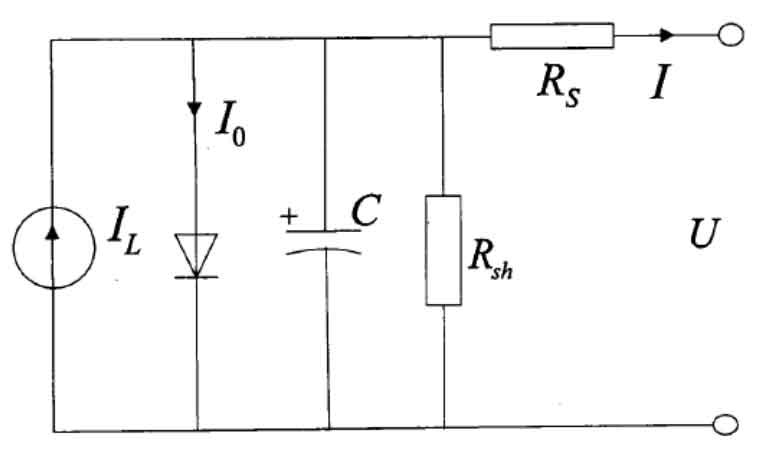
The output current I and voltage U of the photovoltaic cell should meet the mathematical model:
In the formula, I and V represent the output current (A) and voltage (V), respectively; IL is the photogenerated current (A) of the solar photovoltaic cell; I0 is the reverse current (A) of the solar photovoltaic array; Q is the electron charge value, taken as 1.6 × 10⁻¹⁹ (C); K is the Boltzmann constant, taken as 1.38 × 10⁻²³ (J/K); T is the absolute temperature of the solar photovoltaic cell (K); RS and Rsh are the series parallel resistors (Ω) in the circuit, respectively; N1 and n2 are the number of parallel and series solar photovoltaic cells; N is the ideal factor for diodes.
In actual simulation calculations, the parallel resistance Rsh is much greater than the series resistance RS, so the mathematical model of solar photovoltaic cells is often simplified in the industry as follows:
According to the mathematical model of solar photovoltaic cells mentioned above, the corresponding mathematical model expression is analyzed as follows:
The mathematical model of the original solar photovoltaic cell is approximated as the I-U relationship:
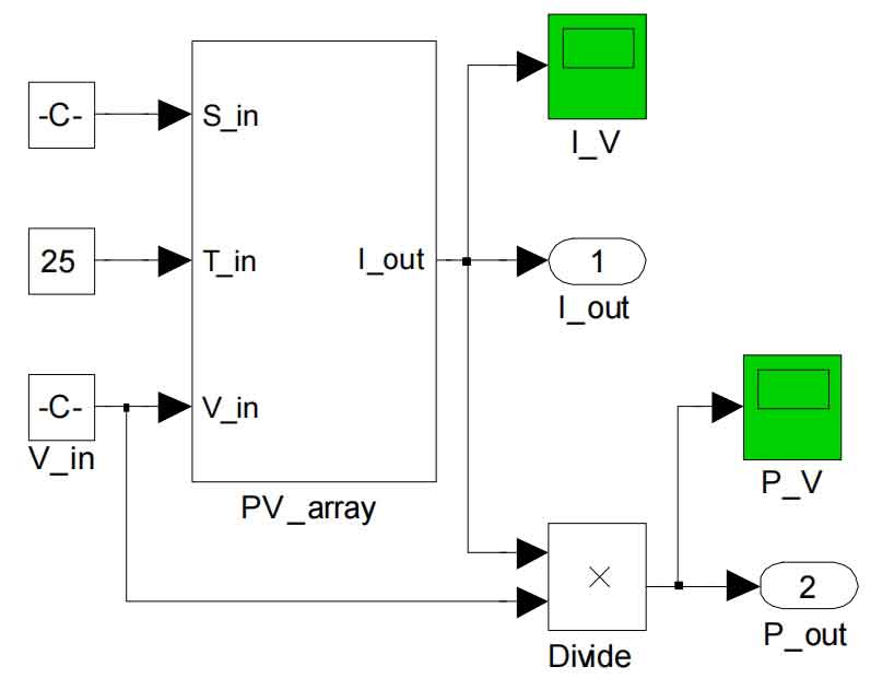
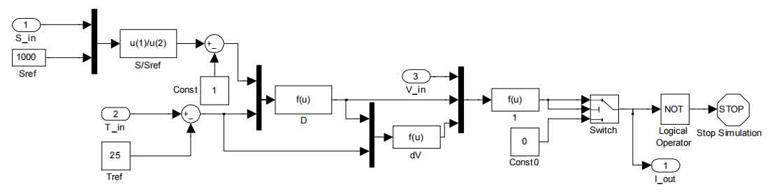
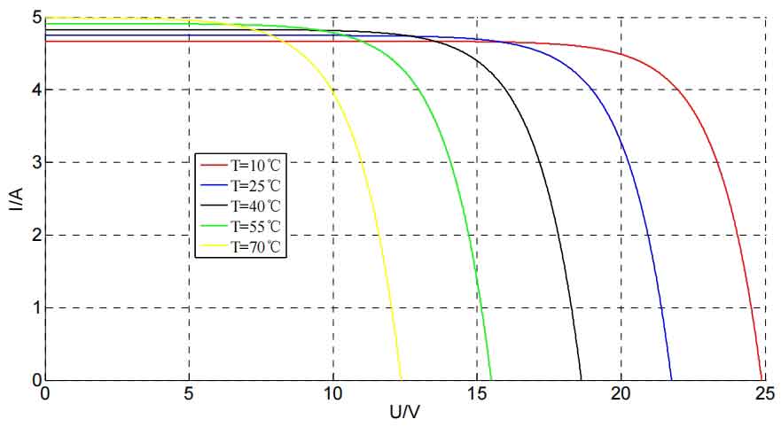
In the formula, Vm, Im, Voc, Isc correspond to the voltage and current at the maximum power point, as well as the open circuit voltage and short circuit current. The values are all from the solar photovoltaic cell manufacturer; T. S refers to the temperature and light intensity input during the actual simulation of solar photovoltaic cells; B1, B2, C, D are all process quantities; a. B is the correction coefficient. Based on the above mathematical model, a simulation model was established using MATLAB Simulink, as shown in Figures 2 and 3. The I-U relationship curves of solar photovoltaic cells can be obtained from the simulation results of Simulink, as shown in Figures 4 and 5. Figure 4 shows the I-U relationship curve under different light intensities at an ambient temperature of 25 ℃; Figure 5 shows the I-U relationship curve under different ambient temperature conditions when the light intensity is 1000W/m2.

1.2 Output characteristics of solar photovoltaic cells
In the actual photovoltaic power generation process, solar photovoltaic cells are highly susceptible to external conditions (such as light, temperature, humidity, etc.). How to achieve maximum power output and continuous high-efficiency operation of solar photovoltaic cells when external conditions change has become an urgent problem to be solved in the photovoltaic power generation industry.
The Maximum Power Point Tracking (MPPT) algorithm is a rising new type of solar photovoltaic control method, gradually replacing traditional solar photovoltaic charge and discharge control methods. Its main purpose is to track the maximum power point of solar photovoltaic cells in real-time, reduce the impact of external conditions on the output efficiency of solar photovoltaic cells, and thereby improve resource utilization.
Based on the existing solar photovoltaic cell models, the P-U relationship curves were obtained through Simulink simulation, as shown in Figures 6 and 7. Figure 6 shows the P-U curves under different light intensities at an ambient temperature of 25 ℃; Figure 7 shows the P-U curves at different ambient temperatures under a light intensity of 1000W/m2.
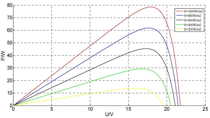

As shown in Figures 6 and 7, the output power of solar photovoltaic cells is influenced by environmental factors such as light intensity and temperature. Therefore, various MPPT control methods have been widely used in modern photovoltaic power generation control systems.
2. Comparison of Three Traditional Maximum Power Tracking Algorithms
At present, the commonly used methods for MPPT control technology include constant voltage method, disturbance observation method, and conductivity increment method. Due to the fact that in the actual operation of photovoltaic systems, the temperature change of solar photovoltaic cells is much smaller than the change in light intensity within a day’s working cycle. Therefore, the following will focus on a brief analysis of several control methods under the condition of light intensity change. The MPPT control principle is shown in Figure 8.
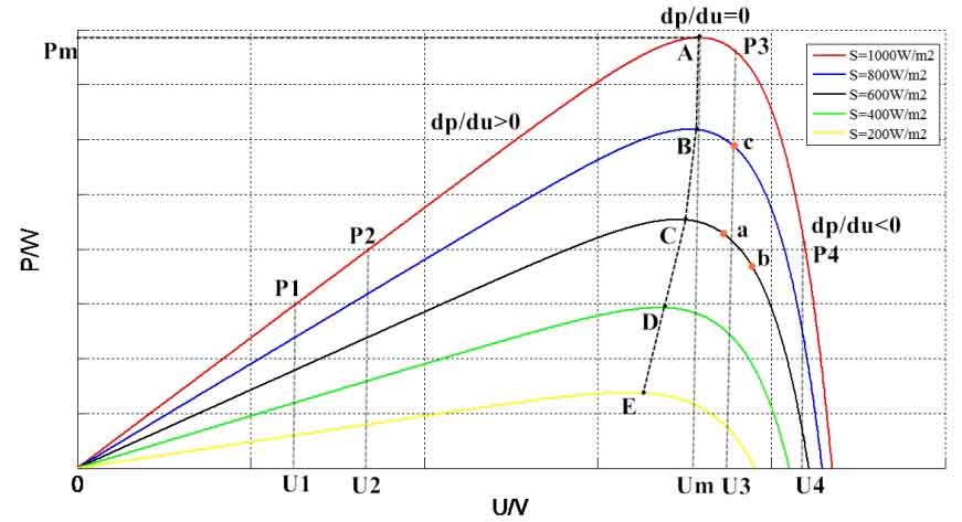
The Constant Voltage Tracking (CVT) method involves controlling the output voltage of the photovoltaic cell at a fixed voltage corresponding to the maximum power point. At this point, the photovoltaic cell operates approximately at the maximum power point throughout the entire working process. From Figure 8, it can be seen that when the temperature effect is ignored, the maximum output power curve of the solar photovoltaic cell is approximately ABCDE under different light intensity conditions, all around the fixed voltage value Um corresponding to the maximum output power. Therefore, if detailed P-U parameters of the region where the photovoltaic array is located are obtained through on-site investigation and testing, the maximum power and corresponding voltage values under each lighting condition can be found through fitting. Then, when the photovoltaic system is working, the corresponding voltage and output power points can be directly matched in real time to quickly and accurately achieve MPP.
The constant voltage method has strong anti-interference ability and stability, can quickly track the maximum power point in real time, and the control is simple and easy to implement. Compared to traditional charge discharge controllers that are directly coupled, the efficiency is improved by more than 20%. However, the constant voltage method is a control method based on ignoring the influence of temperature. When the temperature changes, the voltage corresponding to the maximum power point under each illumination will change to a certain extent. At this time, the power curve can only be re fitted, otherwise it will cause a decrease in efficiency. But re fitting the power curve complicates the control, so this method is gradually unable to adapt to efficient control requirements.
Perturbation and Observation (P&O) method, commonly known as “mountain climbing method”, is a method that changes the disturbance amount of the output voltage. By judging the changes in the output power of the system before and after the disturbance, the output power always moves in the direction of increase. As shown in Figure 8, when the controller gives the system an output voltage disturbance, causing the voltage to change from U1 to U2, the corresponding power also changes from P1 to P2. The direction of the next disturbance is determined by the sign of the difference between the next power P2 and the previous power P1. if Δ If the difference between P (P2-P1) is greater than zero, it indicates that voltage disturbance causes power to change in the direction of increase. The next disturbance direction should maintain the current direction and continue the disturbance; If Δ If P is less than zero, it indicates that voltage disturbance causes power to change in the direction of decrease, and the next disturbance should continue in the opposite direction. At the same time, when the difference between the two is less than a certain quantity, it can be considered as MPP, and its logical diagram is shown in Figure 9. In the figure, P (k-1) and P (k) represent the power that differs by one disturbance cycle.

The disturbance observation method has the advantages of simple control and high maximum power tracking accuracy, but it has three prominent problems. Firstly, the selection of perturbation step size for perturbation observation method is quite difficult; The step size is too large, which shortens the tracking time of the algorithm, but it is prone to overshoot, causing severe oscillations in the entire voltage and power changes, resulting in unnecessary power loss and system instability. If the step size is too small, on the contrary, although it improves the tracking accuracy of the algorithm and reduces power oscillation losses, it will inevitably increase the tracking time and fail to meet the design requirements of fast response for photovoltaic power generation. Secondly, the disturbance observation method actually controls the output power to oscillate around Pm, and cannot make the output power completely equal to Pm. Therefore, it can also cause power oscillation losses and reduce system stability. Thirdly, the perturbation observation method responds slowly to changes in external conditions and is prone to misjudgment. As shown in Figure 8, when the solar photovoltaic cell operates at point a, if the next disturbance increases the disturbance voltage, the power point should move forward to point b. At this point, PbPa, the disturbance will continue to increase the disturbance voltage in the same direction, and the power point will move away from point Pm, which goes against the original intention of the control method and also causes success rate oscillation, causing unnecessary power loss.
The incremental conductivity method (IncCond) is based on the principle that the derivative of power at the maximum power point to voltage is zero, that is:
If P=IV, the formula can be equivalent to:
In practical programming operations, approximating differential calculations as Δ I and Δ V. The formula is equivalent to:
In the formula Δ I and Δ V represents the difference between the current and voltage measured before and after each measurement.
Then I/V in the formula Δ Δ Determine and achieve tracking of the maximum power point. The logical operation diagram of the algorithm is shown in Figure 10.

In the block diagram, V (k-1) and I (k-1) are the voltage and current of the previous cycle, V (k) and I (k) are the voltage and current of the current cycle, I/V is the instantaneous conductivity value collected by the control system, and Vref is the voltage disturbance. According to the logical diagram, define Δ I/ Δ V=0 or Δ I= Δ When V=0, the power point is the maximum power point. Namely Δ I/ Δ When V=- I/V, it indicates that the conductivity collected by the system is equal to the conductivity obtained through the two cycles before and after, which can be considered as maximum power tracking at this time. When Δ V=0 and Δ I> At 0, it indicates that the current is still increasing, and the power point is on the left side of the optimal point. Further disturbance should be added to move the power point towards the current direction; Similarly, when Δ V=0 and Δ When I<0, it indicates that the current is already decreasing, and the power point is on the optimal right side. The disturbance should be reduced to move the power point in the opposite direction. Meanwhile Δ I/ Δ V and instantaneous conductivity – I/V
The principle of comparison is also similar, but it will not be further elaborated here.
By comparing the incremental conductance method with the perturbation observation method, it was found that the two algorithms have certain similarities, but the judgment basis of the incremental conductance method is more complex, which also makes it have higher tracking accuracy. Due to the addition of real-time collected instantaneous conductance as a judgment criterion, it has the ability to adapt to changes in external conditions and reduces the phenomenon of “misjudgment”. However, the incremental conductance method is difficult to meet the judgment criteria for its maximum power point in practical engineering use, so this control method still has the problem of oscillation near the maximum power point. At the same time, this algorithm has more complex judgment conditions and uses instantaneous conductance as the judgment basis, so it also requires higher equipment requirements.
In order to find more efficient algorithms, many experts and scholars have proposed many other improved algorithms on these three traditional algorithms, such as fuzzy logic control, particle swarm optimization, neural network algorithm, gradient method, etc. However, these improved algorithms are only widely discussed in the theoretical field and have not been found to be applied in practical production. Therefore, we will not elaborate on them in detail.