
In the context of global energy transition and the pursuit of carbon neutrality, the role of lithium-ion batteries has become increasingly prominent. As an essential part of renewable energy systems, the energy storage battery is widely used in electric vehicles, grid-scale energy storage, and portable electronics. However, the degradation of battery capacity over repeated charge–discharge cycles is an unavoidable phenomenon that directly affects the safety, reliability, and economic efficiency of energy storage systems. The accurate prediction of the remaining useful life (RUL) of an energy storage battery is therefore a critical task. In this work, I focus on developing an improved stochastic configuration network (SCN) and its optimized version for the life prediction of energy storage batteries. I first analyze the degradation mechanism of lithium-ion batteries, then propose an improved SCN with Laplace regularization, adaptive activation functions, and Gaussian distribution based stochastic parameters. Subsequently, I introduce an improved golden jackal optimization (GJO) algorithm to automatically determine the key hyper-parameters of the model. Extensive experiments on three public battery datasets demonstrate that the proposed hybrid model outperforms several conventional machine learning methods in terms of prediction accuracy and stability.
1. Introduction
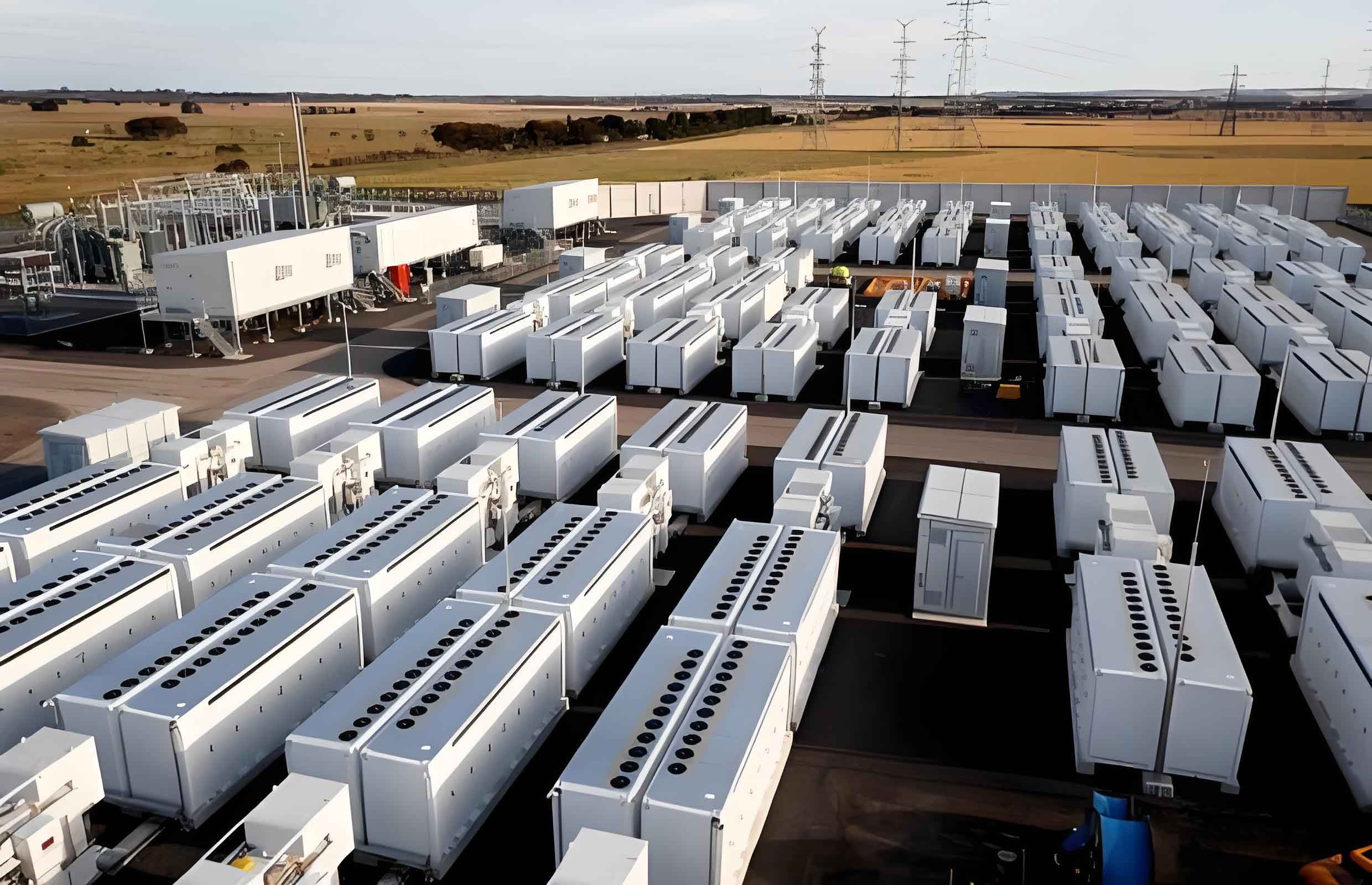
Energy storage batteries, especially lithium-ion batteries, are the core components of modern energy storage systems. Their performance directly influences the operational safety and maintenance cost of the entire system. During their service life, energy storage batteries experience capacity fade, internal resistance increase, and other degradation phenomena. When the available capacity drops below a certain threshold, typically 70% of the rated capacity for many applications, the battery should be replaced to avoid unexpected failures. Therefore, accurate RUL prediction of energy storage batteries is of great significance for proactive maintenance and system reliability.
Existing RUL prediction approaches can be broadly categorized into model-based methods and data-driven methods. Model-based methods rely on electrochemical models, equivalent circuit models, or empirical degradation models. Although these models can describe certain physical mechanisms, they often suffer from high complexity and limited adaptability under varying operating conditions. Data-driven methods, on the other hand, directly learn from historical data without requiring explicit physical knowledge. Common data-driven approaches include autoregressive integrated moving average (ARIMA), support vector regression (SVR), long short-term memory (LSTM) networks, and Gaussian process regression. However, these methods may face issues such as overfitting, sensitivity to hyper-parameters, or poor generalization when applied to different energy storage battery datasets.
In recent years, stochastic configuration network (SCN), proposed by Wang and Li, has attracted increasing attention due to its universal approximation property and fast learning speed. SCN builds a single-hidden-layer feedforward network by incrementally adding hidden nodes under an inequality constraint. The input weights and biases are randomly configured within a data-dependent range, and the output weights are computed by least squares. Compared with traditional random weight networks, SCN provides better generalization and a more compact network structure. However, the original SCN still has limitations when applied to energy storage battery life prediction. In this work, I address these limitations by proposing an improved SCN, referred to as LR-ISCN, which incorporates Gaussian distribution sampling, Cauchy mutation, Laplace regularization, and an adaptive activation function pool. Furthermore, I propose an improved golden jackal optimization (TN-GJO) algorithm to optimize the key parameters of LR-ISCN, forming a hybrid model called TN-GJO-LR-ISCN.
The remainder of this paper is organized as follows. Section 2 presents the degradation mechanism of energy storage batteries and the data preprocessing steps. Section 3 describes the original SCN and the proposed LR-ISCN. Section 4 introduces the improved GJO algorithm and the hybrid TN-GJO-LR-ISCN model. Section 5 presents the experimental setup and results. Section 6 concludes the work.
2. Degradation Mechanism and Data Preprocessing
2.1 Working Principle of Energy Storage Battery
Lithium-ion batteries store and release electrical energy through the reversible intercalation and deintercalation of lithium ions between the positive and negative electrodes. In a typical lithium-ion cell, the positive electrode is composed of materials such as lithium cobalt oxide, lithium iron phosphate, or nickel-manganese-cobalt oxide, while the negative electrode is usually graphite. During the charging process, lithium ions are extracted from the positive electrode and inserted into the negative electrode, while electrons flow through the external circuit. During discharging, the reverse process occurs. The electrolyte, separator, and current collectors play crucial roles in facilitating ion transport and preventing short circuits. The overall reaction can be represented as:
$$ \text{Positive electrode: } \mathrm{LiMO_2} \rightleftharpoons \mathrm{Li_{1-x}MO_2} + x\mathrm{Li^+} + x e^- $$
$$ \text{Negative electrode: } \mathrm{C_6} + x\mathrm{Li^+} + x e^- \rightleftharpoons \mathrm{Li_xC_6} $$
The performance of an energy storage battery degrades with cycling because of side reactions, electrode material degradation, electrolyte decomposition, and lithium plating. These processes lead to loss of active material and increase in internal resistance, which in turn reduce the usable capacity.
2.2 Factors Affecting Battery Degradation
Several factors influence the degradation rate of an energy storage battery, including:
- Charge/discharge cycle number: each cycle causes structural changes in the electrodes and the growth of the solid-electrolyte interface (SEI) layer.
- Over-charge and over-discharge: extreme voltage conditions accelerate side reactions and capacity loss.
- C-rate: high current rates generate heat and mechanical stress, accelerating degradation.
- Temperature: elevated temperatures promote unwanted chemical reactions; low temperatures may cause lithium plating.
- Depth of discharge: deep discharge cycles impose larger stress on the battery.
- Operating voltage window: maintaining the voltage within the recommended range helps extend the battery life.
- Storage conditions: high ambient temperature and high state of charge during storage can increase self-discharge and capacity fade.
Because of these complex interactions, the capacity degradation trajectory is often nonlinear and may exhibit temporary capacity recovery phenomena. This makes accurate RUL prediction challenging.
2.3 Battery Datasets and Preprocessing
In this study, I used three publicly available lithium-ion battery datasets: the CALCE dataset from the Center for Advanced Life Cycle Engineering, the MSTRC dataset from the MIT-Stanford-Toyota Research Center, and the HNEI dataset from the Hawaii Natural Energy Institute. From each dataset, two cells were selected as experimental subjects, resulting in six batteries named A1, A2, C1, C2, H1, and H2. The basic parameters of these batteries are summarized in the following table.
| Dataset | Nominal capacity (Ah) | Charge protocol | Discharge protocol | Environmental temperature (°C) |
|---|---|---|---|---|
| CALCE | 1.35 | 0.5C CC-CV to 4.2V | 0.5C CC to 2.7V | 25 |
| HNEI | 2.8 | C/2 CC | 1.5C CC | 25 |
| MSTRC | 1.1 | One- or two-step fast charging | CC discharge | 30 |
The raw capacity degradation curves often contain noise and outliers caused by measurement errors, sensor malfunction, or capacity regeneration. To improve the data quality, I employed a K-nearest-neighbor (KNN) based outlier removal and imputation method. The Euclidean distance between an abnormal point and its neighboring points is calculated as:
$$ d = \sqrt{\sum_{k=1}^{n} (x_k – \hat{x}_k)^2} $$
where \(x_k\) and \(\hat{x}_k\) are the neighboring points. The weight of each neighbor is computed as:
$$ w_i = \frac{1/d_i}{\sum_{j=1}^{n} 1/d_j} $$
and the missing value is estimated by:
$$ \hat{x} = \sum_{i=1}^{k} w_i x_i $$
After preprocessing, the capacity degradation curves become smoother and more suitable for model training. For each battery, the first 70% of the samples are used as the training set, and the remaining 30% are used as the test set for RUL prediction.
2.4 Evaluation Metrics
To quantitatively evaluate the prediction performance, I adopt three commonly used error metrics: root mean square error (RMSE), mean absolute error (MAE), and mean absolute percentage error (MAPE). Their definitions are given below.
$$ \mathrm{RMSE} = \sqrt{\frac{1}{n} \sum_{i=1}^{n} \left( y_i – \hat{y}_i \right)^2} $$
$$ \mathrm{MAE} = \frac{1}{n} \sum_{i=1}^{n} \left| y_i – \hat{y}_i \right| $$
$$ \mathrm{MAPE} = \frac{1}{n} \sum_{i=1}^{n} \frac{\left| y_i – \hat{y}_i \right|}{y_i} \times 100\% $$
where \(n\) is the number of samples, \(y_i\) is the true capacity value, and \(\hat{y}_i\) is the predicted capacity value. In addition, the RUL prediction error is calculated as the absolute difference between the predicted RUL and the true RUL in terms of the number of cycles.
3. Improved Stochastic Configuration Network for Energy Storage Battery Life Prediction
3.1 Overview of Stochastic Configuration Network
The stochastic configuration network (SCN) is a randomized learning model that incrementally constructs a single-hidden-layer feedforward neural network. Given a training dataset \(\{\mathbf{x}_j, y_j\}_{j=1}^{N}\), where \(\mathbf{x}_j \in \mathbb{R}^d\) and \(y_j \in \mathbb{R}^m\), the output of an SCN with \(L-1\) hidden nodes can be written as:
$$ f_{L-1}(\mathbf{x}) = \sum_{j=1}^{L-1} \beta_j g_j(\mathbf{w}_j^{\mathrm{T}} \mathbf{x} + b_j) $$
where \(g_j(\cdot)\) is the activation function, \(\mathbf{w}_j\) and \(b_j\) are the input weight and bias of the \(j\)-th hidden node, and \(\beta_j\) is the output weight. The residual after \(L-1\) nodes is:
$$ \mathbf{e}_{L-1} = \mathbf{Y} – f_{L-1}(\mathbf{X}) $$
When the residual does not satisfy the stopping criterion, a new hidden node \(g_L(\mathbf{w}_L^{\mathrm{T}} \mathbf{x} + b_L)\) is generated. The random parameters \(\mathbf{w}_L\) and \(b_L\) must satisfy the following inequality constraint:
$$ \left\langle \mathbf{e}_{L-1,q}, g_L(\mathbf{w}_L^{\mathrm{T}} \mathbf{x} + b_L) \right\rangle^2 \geq (1 – r) \delta_{L,q} \| \mathbf{e}_{L-1,q} \|^2, \quad q=1,\dots,m $$
where \(r \in (0,1)\) is a scaling factor, \(\delta_{L,q}\) is a nonnegative sequence, and \(\delta_L = \sum_{q=1}^{m} \delta_{L,q}\) is maximized. After adding the new node, the output weights are recomputed via least squares:
$$ \boldsymbol{\beta}^* = \arg\min_{\boldsymbol{\beta}} \left\| \mathbf{Y} – \mathbf{H}_L \boldsymbol{\beta} \right\|^2 $$
where \(\mathbf{H}_L = [\mathbf{h}_1, \dots, \mathbf{h}_L]\) is the hidden output matrix.
3.2 Limitations of the Original SCN
Although the original SCN performs well on many regression tasks, I observed several drawbacks when applying it to energy storage battery life prediction. First, the random weights and biases are drawn from a uniform distribution, which may not provide sufficient diversity for complex nonlinear degradation patterns. Second, the use of a fixed activation function (e.g., sigmoid) may not be appropriate for all battery datasets. Third, the output weight computation based solely on least squares may lead to overfitting, especially in the later stages of prediction. These issues motivate the development of an improved SCN.
3.3 Proposed LR-ISCN
In this subsection, I present the improved SCN, named LR-ISCN, which incorporates three main modifications.
3.3.1 Gaussian Distribution and Cauchy Mutation
Instead of sampling the input weights \(\mathbf{w}\) and biases \(b\) from a uniform distribution, I use a Gaussian distribution to increase the diversity of the random parameters. The standard Gaussian probability density function is:
$$ f(x) = \frac{1}{\sqrt{2\pi}\sigma} \exp\left( -\frac{(x-\mu)^2}{2\sigma^2} \right) $$
In addition, I introduce a Cauchy mutation operator to further enlarge the random configuration space. The standard Cauchy cumulative distribution function is:
$$ D(x) = \frac{1}{2} + \frac{1}{\pi} \arctan(x), \quad -\infty < x < \infty $$
For an individual \(X\), the Cauchy mutation is performed as:
$$ X_{\mathrm{mutation}} = X + \eta \cdot C(0,1) $$
where \(\eta\) is a scaling constant and \(C(0,1)\) is a random number generated from the standard Cauchy distribution. This operator helps generate new candidate parameters that lead to faster residual reduction, thereby improving the convergence speed and reducing the number of hidden nodes.
3.3.2 Adaptive Activation Function Pool
To overcome the data-dependency problem of a fixed activation function, I construct an activation function pool containing four candidate functions: Sigmoid, Tanh, Gaussian, and Leaky ReLU. Their mathematical definitions are:
$$ \text{Sigmoid}(x) = \frac{1}{1 + e^{-x}} $$
$$ \text{Tanh}(x) = \frac{2}{1 + e^{-2x}} – 1 $$
$$ \text{Gaussian}(x) = \frac{1}{\sqrt{2\pi}} e^{-\frac{x^2}{2}} $$
$$ \text{LeakyReLU}(x) = \max(0.01x, x) $$
Whenever a new hidden node is generated, the proposed algorithm automatically selects the activation function that minimizes the current residual, subject to the same inequality constraint used in SCN. This adaptive mechanism allows the model to fit different energy storage battery datasets more flexibly.
3.3.3 Laplace Regularization
To improve the generalization performance of the model, I add a Laplace regularization term to the output weight objective function. The new optimization problem is:
$$ \boldsymbol{\beta}^* = \arg\min_{\boldsymbol{\beta}} \left\{ \frac{1}{2} \left\| \mathbf{Y} – \mathbf{H} \boldsymbol{\beta} \right\|_F^2 + \frac{\alpha}{2} \mathrm{Tr}\left( \boldsymbol{\beta}^{\mathrm{T}} \mathbf{H}^{\mathrm{T}} \mathbf{L} \mathbf{H} \boldsymbol{\beta} \right) \right\} $$
where \(\mathbf{L}\) is the Laplacian matrix, \(\alpha\) is the regularization coefficient, and \(\mathrm{Tr}(\cdot)\) denotes the trace operator. The solution is:
$$ \boldsymbol{\beta}^* = \left( \mathbf{H}^{\mathrm{T}} \mathbf{H} + \alpha \mathbf{H}^{\mathrm{T}} \mathbf{L} \mathbf{H} \right)^{-1} \mathbf{H}^{\mathrm{T}} \mathbf{Y} $$
The Laplacian matrix is constructed from the similarity matrix \(\mathbf{S}\), where the \((i,j)\)-th element is computed by the Gaussian radial basis function:
$$ S_{ij} = \exp\left( -0.5 \| \mathbf{x}_i – \mathbf{x}_j \|^2 \right) $$
The diagonal degree matrix \(\mathbf{D}\) is defined as:
$$ D_{ii} = \sum_{j=1}^{N} S_{ij} $$
and the Laplacian matrix is:
$$ \mathbf{L} = \mathbf{D}^{-\frac{1}{2}} (\mathbf{D} – \mathbf{S}) \mathbf{D}^{-\frac{1}{2}} $$
This regularization term encodes the local manifold structure of the data, which helps to prevent overfitting and enhances the model’s ability to generalize to unseen battery data.
3.3.4 Algorithm Summary
Let the training set be \(\{\mathbf{X}, \mathbf{Y}\}\), where \(\mathbf{X} \in \mathbb{R}^{N \times d}\) and \(\mathbf{Y} \in \mathbb{R}^{N \times m}\). The LR-ISCN algorithm proceeds as follows.
| Step | Description |
|---|---|
| 1 | Initialize residual \(\mathbf{e}_0 = \mathbf{Y}\), hidden layer output matrix \(\mathbf{H} = []\), and set \(L = 1\). |
| 2 | While \(L \leq L_{\max}\) and \(\|\mathbf{e}_{L-1}\|_F > \varepsilon\): |
| 3 | For each \(\lambda \in \Lambda\), for each candidate trial \(k = 1, 2, \dots, T_{\max}\): randomly generate \(\mathbf{w}_L\) and \(b_L\) from a Gaussian distribution, apply Cauchy mutation, and select the best activation function from the pool. |
| 4 | Compute \(\mathbf{h}_L = g(\mathbf{w}_L^{\mathrm{T}} \mathbf{X} + b_L)\) and the quality score \(\xi_{L,q}\). |
| 5 | If the inequality constraint holds, save the candidate parameters; otherwise, update the scaling factor \(r = r + \tau\) and repeat. |
| 6 | After obtaining the best node parameters, compute the hidden matrix \(\mathbf{H}_L\) and update the output weights using the Laplace-regularized least squares formula. |
| 7 | Update the residual \(\mathbf{e}_L = \mathbf{e}_{L-1} – \mathbf{h}_L \boldsymbol{\beta}_L\) and increment \(L\). |
| 8 | Return the final output weights \(\boldsymbol{\beta}^*\) and the hidden node parameters. |
3.4 Simulation Results of LR-ISCN vs SCN
I conducted comparative experiments on six batteries using the original SCN and the proposed LR-ISCN. The maximum number of hidden nodes \(L_{\max}\) was set to 25 and 50 in two separate test groups. The maximum number of random candidates \(T_{\max}\) was 100, and the tolerance \(\varepsilon\) was 0.001. All results were averaged over 10 independent runs. The training errors of both algorithms on battery A1 are illustrated in the convergence curves, which are not reproduced here due to the text-only format. The key observation is that LR-ISCN consistently achieves lower training errors and faster convergence than SCN. Moreover, when \(L_{\max}=50\), LR-ISCN often stops training early with fewer than 50 hidden nodes, indicating a more compact network structure.
The following tables summarize the performance comparison on the CALCE dataset for the two settings. It can be seen that LR-ISCN outperforms SCN in both training and testing phases on both batteries.
| Battery | Metric | Training SCN | Training LR-ISCN | Testing SCN | Testing LR-ISCN |
|---|---|---|---|---|---|
| A1 | RMSE | 2.5019E-03 | 9.8268E-04 | 8.8806E-03 | 3.0838E-03 |
| MAE | 1.6879E-03 | 7.3325E-04 | 5.1314E-03 | 2.3004E-03 | |
| MAPE | 1.3704E-01 | 6.0068E-02 | 4.9592E-01 | 2.1896E-01 | |
| A2 | RMSE | 2.8138E-03 | 9.4958E-04 | 2.8981E-02 | 3.9203E-03 |
| MAE | 1.9072E-03 | 6.9359E-04 | 1.2376E-02 | 2.6537E-03 | |
| MAPE | 1.5545E-01 | 5.8132E-02 | 1.1974E+00 | 2.5238E-01 |
| Battery | Metric | Training SCN | Training LR-ISCN | Testing SCN | Testing LR-ISCN |
|---|---|---|---|---|---|
| A1 | RMSE | 2.4804E-03 | 9.5089E-04 | 9.3136E-03 | 2.0520E-03 |
| MAE | 1.6764E-03 | 7.2179E-04 | 6.5007E-03 | 1.5653E-03 | |
| MAPE | 1.3617E-01 | 5.9135E-02 | 6.2253E-01 | 1.4859E-01 | |
| A2 | RMSE | 2.7809E-03 | 9.4934E-04 | 2.0120E-02 | 6.5995E-03 |
| MAE | 1.8694E-03 | 6.9165E-04 | 8.2770E-03 | 4.1939E-03 | |
| MAPE | 1.5245E-01 | 5.7963E-02 | 8.0017E-01 | 4.0045E-01 |
Similar improvements were observed on the MSTRC and HNEI datasets. In most cases, LR-ISCN provided lower RMSE, MAE, and MAPE than SCN. Although there were a few exceptions where SCN had slightly better values on some metrics, the differences were negligible. The overall trend confirms the effectiveness of the proposed modifications.
4. Optimization of LR-ISCN Using Improved Golden Jackal Optimization
4.1 Golden Jackal Optimization Algorithm
The golden jackal optimization (GJO) algorithm is a recent nature-inspired metaheuristic algorithm based on the cooperative hunting behavior of male and female golden jackals. It maintains a population of candidate solutions (preys) and updates their positions in two phases: exploration and exploitation. The position update formulas are:
$$ Y_1(t) = Y_M(t) – E \cdot | rl \cdot \mathrm{Prey}(t) – Y_M(t) | $$
$$ Y_2(t) = Y_{FM}(t) – E \cdot | rl \cdot \mathrm{Prey}(t) – Y_{FM}(t) | $$
$$ Y(t+1) = \frac{Y_1(t) + Y_2(t)}{2} $$
where \(Y_M\) and \(Y_{FM}\) are the positions of the male and female jackals, \(E\) is the prey’s escape energy, and \(rl\) is a random vector based on the Levy flight distribution:
$$ rl = 0.05 \cdot LF(y) $$
$$ LF(y) = 0.01 \cdot \frac{u \cdot \sigma}{|v|^{1/\beta}}, \quad \sigma = \left( \frac{\Gamma(1+\beta) \sin(\pi \beta / 2)}{\Gamma((1+\beta)/2) \cdot \beta \cdot 2^{(\beta-1)/2}} \right)^{1/\beta} $$
The escape energy \(E\) is modeled as:
$$ E = E_0 \cdot E_1, \quad E_0 = 2 \cdot \mathrm{rand} – 1, \quad E_1 = c_1 \cdot \left( 1 – \frac{t}{T} \right) $$
where \(c_1 = 1.5\) in the original version.
4.2 Improved GJO (TN-GJO)
The original GJO algorithm has some drawbacks, such as slow convergence in the later iterations and a tendency to fall into local optima. To address these issues, I propose an improved version, named TN-GJO, which incorporates two main enhancements.
4.2.1 Tent Chaotic Mapping for Population Initialization
In order to enhance the diversity of the initial population, I employ Tent chaotic mapping to generate the initial positions of the preys. The Tent map is defined as:
$$ z_{k+1} = \begin{cases} \frac{z_k}{\mu}, & 0 < z_k \leq \mu \\ \frac{1 – z_k}{1 – \mu}, & \mu < z_k \leq 1 \end{cases} $$
The chaotic sequence is then transformed to the search space by:
$$ x_k = x_{\min} + z_k (x_{\max} – x_{\min}) $$
This mapping provides a more uniform distribution of the initial population compared with pure random initialization.
4.2.2 Nonlinear Energy Parameter
In the original GJO, the energy parameter \(E_1\) decreases linearly, which may cause the algorithm to be trapped in local optima during the later iterations. I modify the expression to a nonlinear decreasing form:
$$ E_1 = c_1 \cdot \left( 1 – \frac{t}{T} \right)^3 $$
This nonlinear decay balances the global search (exploration) and local search (exploitation) abilities more effectively. The improved algorithm is summarized in the following pseudo-code table.
| Step | Operation |
|---|---|
| 1 | Initialize the population size \(N\), maximum iterations \(T\), and generate initial prey positions using Tent chaotic mapping. |
| 2 | Evaluate the fitness of each prey and identify the best (male) and second-best (female) jackal positions. |
| 3 | For each iteration \(t=1,\dots,T\): |
| 4 | Update the escape energy \(E\) using the nonlinear formula. |
| 5 | If \(|E| \geq 1\), update positions using the exploration equations; otherwise, use the exploitation equations. |
| 6 | Combine the male and female updated positions to obtain the new prey position. |
| 7 | After the population update, go to the next iteration until the stopping criterion is met. |
4.3 Hybrid TN-GJO-LR-ISCN Model
In the LR-ISCN model, the scaling factor \(r\) and the random parameter range \(\lambda\) significantly influence the network performance. These hyper-parameters are usually chosen manually, which is inefficient and may lead to suboptimal results. To overcome this, I utilize the proposed TN-GJO algorithm to automatically optimize \(r\) and \(\lambda\). The fitness function is defined as the RMSE of the LR-ISCN model on the training set:
$$ f = \sqrt{\frac{1}{K} \sum_{i=1}^{K} \left( y_i – \hat{y}_i \right)^2} $$
The optimization process searches for the values of \(r\) and \(\lambda\) that minimize this fitness function. The steps of the combined approach, denoted as TN-GJO-LR-ISCN, are as follows:
- Initialize TN-GJO parameters (population size, maximum iterations, bounds of \(r\) and \(\lambda\), Tent chaos parameter).
- Generate the initial population of (\(r\), \(\lambda\)) using Tent chaos.
- For each individual, construct and train an LR-ISCN model; compute the fitness value using the RMSE.
- Update the jackal positions according to the TN-GJO rules.
- Repeat until the stopping criterion is satisfied; output the optimal \(r\) and \(\lambda\).
- Train the final LR-ISCN model with the optimal parameters and perform energy storage battery RUL prediction.
5. Experimental Results and Discussion
5.1 Experimental Setup
Experiments were carried out on the six batteries from the three datasets. For each battery, the first 70% of the normalized capacity data were used for training, and the remaining 30% were used for testing. The input features included voltage, current, and internal resistance, while the output was the battery capacity. All models were run 10 times, and the average results were recorded.
For the LR-ISCN model, the maximum number of hidden nodes was set to 50, the maximum number of random candidates was 100, and the tolerance was 0.001. For TN-GJO, the population size was set to 10 and the maximum number of iterations was 20. The bounds for \(r\) and \(\lambda\) were set to [0.1, 0.9] and [0.5, 1.0], respectively.
5.2 Comparison of TN-GJO-LR-ISCN with LR-ISCN
The training convergence curves and the prediction results on the CALCE batteries are very illustrative. The TN-GJO-LR-ISCN model always converged faster than LR-ISCN in terms of the training RMSE and usually required fewer hidden nodes to reach the same error level. For example, on battery A1, the TN-GJO-LR-ISCN stopped after generating 41 hidden nodes, while LR-ISCN needed more than 50 nodes. This indicates that the optimized hyper-parameters lead to a more compact network structure.
The following table compares the RUL prediction errors for all six batteries between LR-ISCN and TN-GJO-LR-ISCN.
| Battery | True RUL | LR-ISCN predicted RUL | LR-ISCN error | TN-GJO-LR-ISCN predicted RUL | TN-GJO-LR-ISCN error |
|---|---|---|---|---|---|
| A1 | 76 | 79 | 3 | 76 | 0 |
| A2 | 75 | 72 | 3 | 75 | 0 |
| C1 | 245 | 226 | 19 | 243 | 2 |
| C2 | 307 | 277 | 30 | 300 | 7 |
| H1 | 34 | 22 | 12 | 30 | 4 |
| H2 | 19 | 18 | 1 | 18 | 1 |
It is evident that TN-GJO-LR-ISCN significantly reduces the RUL prediction error for most batteries. For battery A1 and A2, the error becomes zero, meaning the model exactly predicts the true remaining life.
5.3 Comparison with Conventional Machine Learning Models
To further validate the superiority of the proposed model, I compared TN-GJO-LR-ISCN with three widely used methods: ARIMA, SVR, and LSTM. The evaluation metrics on the CALCE dataset are shown in the following table.
| Battery | Metric | ARIMA | SVR | LSTM | TN-GJO-LR-ISCN |
|---|---|---|---|---|---|
| A1 | RMSE | 9.7879E-03 | 6.9805E-03 | 2.3041E-02 | 2.6361E-03 |
| MAE | 8.0176E-03 | 5.6104E-03 | 2.1570E-02 | 1.9335E-03 | |
| MAPE | 7.5627E-01 | 5.2430E-01 | 2.0486E+00 | 1.8424E-01 | |
| RUL error | 21 | 18 | 56 | 0 | |
| A2 | RMSE | 1.8065E-02 | 1.1433E-02 | 1.2435E-02 | 2.4838E-03 |
| MAE | 1.4413E-02 | 9.3745E-03 | 1.0065E-02 | 1.8750E-03 | |
| MAPE | 1.3374E+00 | 8.7246E-01 | 9.4731E-01 | 1.7544E-01 | |
| RUL error | 16 | 9 | 11 | 0 |
On the MSTRC dataset, ARIMA, SVR, and LSTM all failed to predict the RUL for batteries C1 and C2 in some cases, whereas TN-GJO-LR-ISCN successfully predicted the RUL with errors of 2 and 7 cycles, respectively. The detailed metrics are given below.
| Battery | Metric | ARIMA | SVR | LSTM | TN-GJO-LR-ISCN |
|---|---|---|---|---|---|
| C1 | RMSE | 8.0643E-03 | 1.0181E-01 | 2.4811E-02 | 1.9515E-03 |
| MAE | 6.7363E-03 | 9.3445E-02 | 1.8746E-02 | 1.8592E-03 | |
| MAPE | 6.9866E-01 | 9.7813E+00 | 1.9965E+00 | 1.9062E-01 | |
| RUL error | Not observed | Not observed | Not observed | 2 | |
| C2 | RMSE | 4.7973E-02 | 1.0609E-01 | 3.4497E-02 | 1.7096E-03 |
| MAE | 3.4128E-02 | 9.5471E-02 | 2.8343E-02 | 1.2037E-03 | |
| MAPE | 3.6630E+00 | 1.0008E+01 | 3.0002E+00 | 1.2763E-01 | |
| RUL error | Not observed | Not observed | Not observed | 7 |
For the HNEI dataset, the proposed model also yields the best results. The following table summarizes the performance comparisons.
| Battery | Metric | ARIMA | SVR | LSTM | TN-GJO-LR-ISCN |
|---|---|---|---|---|---|
| H1 | RMSE | 7.8031E-02 | 1.4611E-02 | 2.6139E-02 | 9.7018E-03 |
| MAE | 6.4655E-02 | 1.0344E-02 | 2.4405E-02 | 6.0072E-03 | |
| MAPE | 2.9331E+00 | 4.6832E-01 | 1.1048E+00 | 2.7086E-01 | |
| RUL error | 16 | 4 | 5 | 4 | |
| H2 | RMSE | 8.9648E-02 | 1.6482E-02 | 2.9191E-02 | 6.5937E-03 |
| MAE | 7.4947E-02 | 1.1545E-02 | 2.5578E-02 | 6.0389E-03 | |
| MAPE | 3.4187E+00 | 5.2581E-01 | 1.1682E+00 | 2.7343E-01 | |
| RUL error | 8 | 3 | 4 | 1 |
All experimental results consistently demonstrate that TN-GJO-LR-ISCN achieves the highest prediction accuracy among the compared methods. The improvement is particularly remarkable for the MSTRC dataset, where the conventional methods cannot even provide a valid RUL prediction. The proposed model not only captures the nonlinear degradation trend but also mitigates the overfitting phenomenon often observed in the latter stage of prediction.
6. Conclusion
In this work, I have presented a comprehensive study on the life prediction of energy storage batteries using an improved stochastic configuration network and its optimized version. The main contributions are as follows:
- I proposed an improved SCN (LR-ISCN) that uses Gaussian distribution and Cauchy mutation for generating random input parameters, an adaptive activation function pool for flexible nonlinear mapping, and Laplace regularization for output weight computation. This model significantly enhances the generalization performance and reduces the network complexity compared with the original SCN.
- I proposed an improved golden jackal optimization algorithm (TN-GJO) by introducing Tent chaotic mapping for population initialization and a nonlinear energy parameter for better exploration-exploitation balance. TN-GJO effectively avoids local optima and accelerates convergence.
- I integrated TN-GJO with LR-ISCN to automatically determine the crucial hyper-parameters (\(r\) and \(\lambda\)), resulting in a hybrid model TN-GJO-LR-ISCN that achieves accurate and stable RUL prediction for energy storage batteries.
- Extensive experiments on three public battery datasets demonstrate that TN-GJO-LR-ISCN outperforms ARIMA, SVR, LSTM, and the non-optimized LR-ISCN in terms of RMSE, MAE, MAPE, and RUL prediction error.
Despite the encouraging results, the proposed model may still face challenges in extremely large-scale and highly dynamic battery systems. Future work will focus on developing more efficient training strategies and integrating online learning mechanisms to further improve the adaptability of the model. In addition, exploring the combination of the proposed method with other ensemble techniques or transfer learning approaches could be a promising direction for cross-dataset and cross-condition battery life prediction.